사람들은 새로운 프로그래밍 언어를 만들 때 이전 언어의 좋은 기능을 유지하고 나쁜 것은 수정하기를 원하기 때문에 그렇게합니다.
이런 의미에서 Guido van Rossum은 ABC를 개선하기 위해 1980 년대 후반에 Python을 만들었습니다. 후자는너무 완벽 해프로그래밍 언어의 경우-강성으로 인해 쉽게 가르 칠 수 있었지만 실제 생활에서는 사용하기 어려웠습니다.
대조적으로 Python은 매우 실용적입니다. 당신은 이것을에서 볼 수 있습니다파이썬의 선, 제작자의 의도를 반영합니다.
못생긴 것보다 아름다운 것이 낫습니다.
명시적인 것이 암시적인 것보다 낫습니다.
단순한 것이 복잡한 것보다 낫습니다.
복잡한 것이 복잡한 것보다 낫습니다.
플랫이 중첩보다 낫습니다.
스파 스는 조밀 한 것보다 낫습니다.
가독성이 중요합니다.
특별한 경우는 규칙을 어길만큼 특별하지 않습니다.
실용성이 순결을 능가하지만.
[...]
Python은 여전히 ABC의 좋은 기능인 가독성, 단순성, 초보자 친화적 인 기능을 유지했습니다. 그러나 Python은 ABC보다 훨씬 더 강력하고 실제 생활에 적합합니다.
ABC는 줄리아를위한 길을 닦고있는 파이썬을위한 길을 열었습니다. ~의 사진데이비드 발류의 위에Unsplash
같은 의미에서 Julia의 제작자는 다른 언어의 좋은 부분은 유지하고 나쁜 언어는 버리기를 원합니다. 그러나 Julia는 훨씬 더 야심적입니다. 하나의 언어를 대체하는 대신 모든 언어를 이기고 싶습니다.
우리는 더 많은 것을 원합니다.우리는 자유 라이선스가있는 오픈 소스 언어를 원합니다. Ruby의 역동 성과 함께 C의 속도를 원합니다. Lisp와 같은 진정한 매크로를 사용하지만 Matlab과 같은 명확하고 친숙한 수학적 표기법을 사용하는 동음이의 언어를 원합니다. 우리는 Python처럼 일반 프로그래밍에 유용하고, R만큼 쉬운 통계, Perl만큼 자연스러운 문자열 처리, Matlab처럼 선형 대수에 대해 강력하고, 프로그램을 셸처럼 결합하는 데 능숙한 것을 원합니다. 배우기 쉽지만 가장 심각한 해커를 행복하게 만드는 것. 우리는 그것이 상호 작용하고 컴파일되기를 원합니다.
Julia는 현재 존재하는 모든 장점을 혼합하고 다른 언어의 단점과 교환하지 않기를 원합니다. Julia는 어린 언어이지만 이미 제작자가 설정 한 많은 목표를 달성했습니다.
Julia 개발자가 좋아하는 것
다재
Julia는 간단한 기계 학습 응용 프로그램에서 거대한 슈퍼 컴퓨터 시뮬레이션에 이르기까지 모든 것에 사용할 수 있습니다. 어느 정도까지는 파이썬도이 작업을 수행 할 수 있습니다. 그러나 파이썬은 어떻게 든 그 일로 성장했습니다.
이것은 Python의 가장 강력한 포인트 중 하나입니다. 관리가 잘되는 수많은 라이브러리입니다. Julia는 라이브러리가 많지 않으며 사용자는 (아직) 놀라 울 정도로 관리되지 않는다고 불평했습니다.
그러나 Julia가 제한된 리소스를 가진 아주 어린 언어라고 생각할 때 이미 보유하고있는 라이브러리의 수는 매우 인상적입니다. Julia의 라이브러리 양이 증가하고 있다는 사실 외에도 예를 들어 C 및 Fortran의 라이브러리와 인터페이스하여 플롯을 처리 할 수 있습니다.
동적 및 정적 유형
Python은 100 % 동적으로 입력됩니다. 이것은 프로그램이 런타임에 변수가 실수인지 정수인지를 결정한다는 것을 의미합니다.
이것은 매우 초보자에게 친숙하지만 가능한 버그가 많이 발생합니다. 이는 가능한 모든 시나리오에서 Python 코드를 테스트해야 함을 의미합니다. 이는 많은 시간이 걸리는 매우 멍청한 작업입니다.
Julia 제작자도 배우기 쉽기를 원했기 때문에 Julia는 동적 타이핑을 완벽하게 지원합니다. 그러나 Python과 달리, 원하는 경우 정적 유형을 도입 할 수 있습니다. 예를 들어 C 또는 Fortran에있는 방식으로 제공됩니다.
이렇게하면 엄청난 시간을 절약 할 수 있습니다.테스트하지 않은 것에 대한 변명코드에서 의미가있는 곳에 유형을 지정할 수 있습니다.
이 모든 것들이 꽤 훌륭하게 들리지만 Julia는 Python에 비해 여전히 작다는 것을 명심하는 것이 중요합니다.
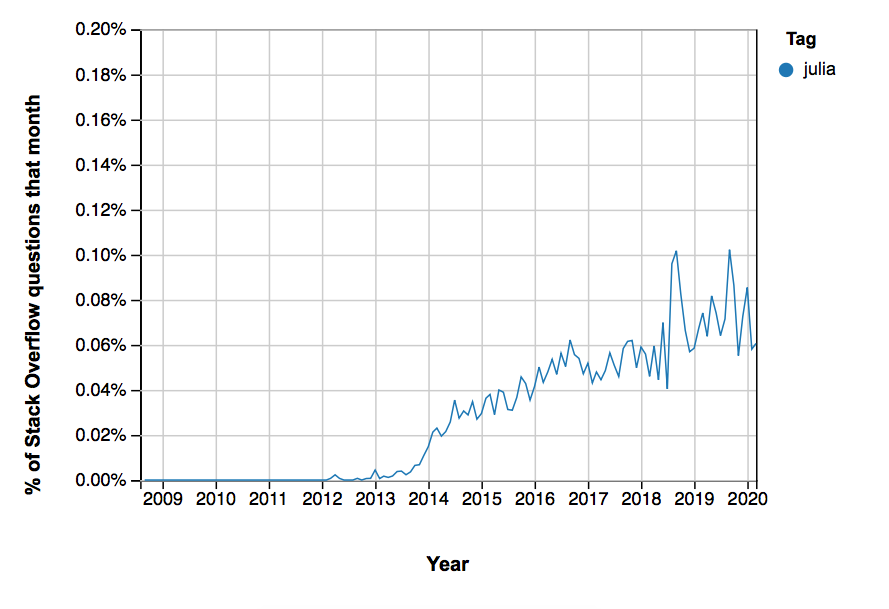
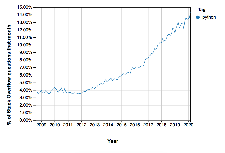
꽤 좋은 지표 중 하나는 StackOverflow에 대한 질문 수입니다.이 시점에서 Python은 Julia보다 약 20 개 더 자주 태그가 지정됩니다!
이것은 Julia가 인기가 없다는 것을 의미하는 것이 아니라 프로그래머가 채택하는 데 자연스럽게 시간이 걸립니다.
생각해보십시오. 전체 코드를 다른 언어로 작성하고 싶습니까? 아니요, 차라리 향후 프로젝트에서 새로운 언어를 시도하고 싶습니다. 이로 인해 모든 프로그래밍 언어가 출시와 채택 사이에 직면하는 시간 지연이 발생합니다.
하지만 지금 채택한다면 (Julia는 엄청난 양의 언어 변환을 허용하기 때문에 쉽습니다.) 미래에 투자하는 것입니다. 점점 더 많은 사람들이 Julia를 채택함에 따라 이미 질문에 답할 수있는 충분한 경험을 쌓을 것입니다. 또한 점점 더 많은 Python 코드가 Julia로 대체됨에 따라 코드의 내구성이 향상됩니다.
40 년 전 인공 지능은 틈새 현상에 불과했습니다. 업계와 투자자들은 그것을 믿지 않았고 많은 기술이 투박하고 사용하기 어려웠습니다. 하지만 그 당시 배운 사람들은 오늘날의 거인입니다. 수요가 너무 많아서그들의 급여NFL 선수와 일치합니다.
마찬가지로 Julia는 지금도 여전히 매우 틈새 시장입니다. 그러나 그것이 커지면 큰 승자는 일찍 채택한 사람들이 될 것입니다.
지금 Julia를 입양하면 10 년 안에 엄청난 돈을 벌 수 있다는 말이 아닙니다. 하지만 기회가 늘어나고 있습니다.
생각해보십시오. 대부분의 프로그래머는 CV에 Python을 사용합니다. 그리고 앞으로 몇 년 안에 우리는 취업 시장에서 더 많은 Python 프로그래머를 보게 될 것입니다. 그러나 Python에 대한 기업의 수요가 느려지면 Python 프로그래머의 관점은 떨어질 것입니다. 처음에는 느리지 만 불가피합니다.
반면에 Julia를 이력서에 올릴 수 있다면 진정한 우위를 점할 수 있습니다. 솔직히 말해서 다른 Pythonista와 다른 점은 무엇입니까? 별로. 하지만 3 년 안에 줄리아 프로그래머는 그리 많지 않을 것입니다.
Julia-skills를 사용하면 직업 요구 사항 이상의 관심사가 있음을 보여줄뿐만 아니라 또한 배우고 자하는 열의와 프로그래머가된다는 것이 무엇을 의미하는지에 대해 더 넓은 이해를 갖고 있음을 보여줍니다. 즉, 당신은 그 일에 적합합니다.
여러분과 다른 Julia 프로그래머는 미래의 록 스타이며 여러분도 알고 있습니다. 또는Julia의 제작자2012 년에 이렇게 말했습니다.
우리가 용납 할 수없는 욕심이 많다는 것을 알고 있지만 우리는 여전히 모든 것을 갖고 싶어합니다. 약 2 년 반 전에 우리는 탐욕의 언어를 만들기 시작했습니다. 완전하지는 않지만 1.0 릴리즈를 할 때입니다. 우리가 만든 언어는줄리아. 그것은 이미 우리의 불의한 요구의 90 %를 제공하고 있으며, 이제는 그것을 더 구체화하기 위해 다른 사람들의 불의한 요구가 필요합니다. 그래서 만약 당신이 탐욕스럽고 비합리적이고 까다로운 프로그래머라면, 우리는 당신이 시도해보기를 바랍니다.
파이썬은 여전히 미친 듯이 인기가 있습니다. 그러나 지금 Julia를 배우면 나중에 황금 티켓이 될 수 있습니다. 이런 의미에서 : Bye-bye Python. 안녕하세요 Julia!
If Julia is still a mystery to you, don’t worry. Photo by Julia Caesar on Unsplash
Don’t get me wrong. Python’s popularity is still backed by a rock-solid community of computer scientists, data scientists and AI specialists.
But if you’ve ever been at a dinner table with these people, you also know how much they rant about the weaknesses of Python. From being slow to requiring excessive testing, to producing runtime errors despite prior testing — there’s enough to be pissed off about.
Which is why more and more programmers are adopting other languages — the top players being Julia, Go, and Rust. Julia is great for mathematical and technical tasks, while Go is awesome for modular programs, and Rust is the top choice for systems programming.
Since data scientists and AI specialists deal with lots of mathematical problems, Julia is the winner for them. And even upon critical scrutiny, Julia has upsides that Python can’t beat.
When people create a new programming language, they do so because they want to keep the good features of old languages and fix the bad ones.
In this sense, Guido van Rossum created Python in the late 1980s to improve ABC. The latter was too perfect for a programming language — while its rigidity made it easy to teach, it was hard to use in real life.
In contrast, Python is quite pragmatic. You can see this in the Zen of Python, which reflects the intention that the creators have:
Beautiful is better than ugly.
Explicit is better than implicit.
Simple is better than complex.
Complex is better than complicated.
Flat is better than nested.
Sparse is better than dense.
Readability counts.
Special cases aren't special enough to break the rules.
Although practicality beats purity.
[...]
Python still kept the good features of ABC: Readability, simplicity, and beginner-friendliness for example. But Python is far more robust and adapted to real life than ABC ever was.
ABC paved the way for Python, which is paving the way for Julia. Photo by David Ballew on Unsplash
In the same sense, the creators of Julia want to keep the good parts of other languages and ditch the bad ones. But Julia is a lot more ambitious: instead of replacing one language, it wants to beat them all.
We are greedy: we want more.We want a language that's open source, with a liberal license. We want the speed of C with the dynamism of Ruby. We want a language that's homoiconic, with true macros like Lisp, but with obvious, familiar mathematical notation like Matlab. We want something as usable for general programming as Python, as easy for statistics as R, as natural for string processing as Perl, as powerful for linear algebra as Matlab, as good at gluing programs together as the shell. Something that is dirt simple to learn, yet keeps the most serious hackers happy. We want it interactive and we want it compiled.
Julia wants to blend all upsides that currently exist, and not trade them off for the downsides in other languages. And even though Julia is a young language, it has already achieved a lot of the goals that the creators set.
What Julia developers are loving
Versatility
Julia can be used for everything from simple machine learning applications to enormous supercomputer simulations. To some extent, Python can do this, too — but Python somehow grew into the job.
In contrast, Julia was built precisely for this stuff. From the bottom up.
Speed
Julia’s creators wanted to make a language that is as fast as C — but what they created is even faster. Even though Python has become easier to speed up in recent years, its performance is still a far cry from what Julia can do.
In 2017, Julia even joined the Petaflop Club — the small club of languages who can exceed speeds of one petaflop per second at peak performance. Apart from Julia, only C, C++ and Fortran are in the club right now.
With its more than 30 years of age, Python has an enormous and supportive community. There is hardly a Python-related question that you can’t get answered within one Google search.
In contrast, the Julia community is pretty tiny. While this means that you might need to dig a bit further to find an answer, you might link up with the same people again and again. And this can turn into programmer-relationships that are beyond value.
Code conversion
You don’t even need to know a single Julia-command to code in Julia. Not only can you use Python and C code within Julia. You can even use Julia within Python!
Needless to say, this makes it extremely easy to patch up the weaknesses of your Python code. Or to stay productive while you’re still getting to know Julia.
Libraries are still a strong point of Python. Photo by Susan Yin on Unsplash
Libraries
This is one of the strongest points of Python — its zillion well-maintained libraries. Julia doesn’t have many libraries, and users have complained that they’re not amazingly maintained (yet).
But when you consider that Julia is a very young language with a limited amount of resources, the number of libraries that they already have is pretty impressive. Apart from the fact that Julia’s amount of libraries is growing, it can also interface with libraries from C and Fortran to handle plots, for example.
Dynamic and static types
Python is 100% dynamically typed. This means that the program decides at runtime whether a variable is a float or an integer, for example.
While this is extremely beginner-friendly, it also introduces a whole host of possible bugs. This means that you need to test Python code in all possible scenarios — which is quite a dumb task that takes a lot of time.
Since the Julia-creators also wanted it to be easy to learn, Julia fully supports dynamical typing. But in contrast to Python, you can introduce static types if you like — in the way they are present in C or Fortran, for example.
This can save you a ton of time: Instead of finding excuses for not testing your code, you can specify the type wherever it makes sense.
Number of questions tagged Julia (left) and Python (right) on StackOverflow.
While all these things sound pretty great, it’s important to keep in mind that Julia is still tiny compared to Python.
One pretty good metric is the number of questions on StackOverflow: At this point in time, Python is tagged about twenty more often than Julia!
This doesn’t mean that Julia is unpopular — rather, it’s naturally taking some time to get adopted by programmers.
Think about it — would you really want to write your whole code in a different language? No, you’d rather try a new language in some future project. This creates a time lag that every programming language faces between its release and its adoption.
But if you adopt it now — which is easy because Julia allows an enormous amount of language conversion — you’re investing in the future. As more and more people adopt Julia, you’ll already have gained enough experience to answer their questions. Also, your code will be more durable as more and more Python code is replaced by Julia.
Forty years ago, artificial intelligence was nothing but a niche phenomenon. The industry and investors didn’t believe in it, and many technologies were clunky and hard to use. But those who learned it back then are the giants of today — those that are so high in demand that their salary matches that of an NFL player.
Similarly, Julia is still very niche now. But when it grows, the big winners will be those who adopted it early.
I’m not saying that you’re guaranteed to make a shitload of money in ten years if you adopt Julia now. But you’re increasing your chances.
Think about it: Most programmers out there have Python on their CV. And in the next few years, we’ll see even more Python programmers on the job market. But if the demand of enterprises for Python slows, the perspectives for Python programmers are going to go down. Slowly at first, but inevitably.
On the other hand, you have a real edge if you can put Julia on your CV. Because let’s be honest, what distinguishes you from any other Pythonista out there? Not much. But there won’t be that many Julia-programmers out there, even in three years’ time.
With Julia-skills, not only are you showing that you have interests beyond the job requirements. You’re also demonstrating that you’re eager to learn and that you have a broader sense of what it means to be a programmer. In other words, you’re fit for the job.
You — and the other Julia programmers — are future rockstars, and you know it. Or, as Julia’s creators said it in 2012:
Even though we recognize that we are inexcusably greedy, we still want to have it all. About two and a half years ago, we set out to create the language of our greed. It's not complete, but it's time for a 1.0 release — the language we've created is called Julia. It already delivers on 90% of our ungracious demands, and now it needs the ungracious demands of others to shape it further. So, if you are also a greedy, unreasonable, demanding programmer, we want you to give it a try.
Python is still insanely popular. But if you learn Julia now, that could be your golden ticket later on. In this sense: Bye-bye Python. Hello Julia!
Coding efficiently is one of the key premises to the use case of Python and Lambda expressions are no different. Python lambda’s are anonymous functions which involve small and concise syntax, whereas at times, regular functions can be too descriptive and quite long.
Python is one of a few languages which had lambda functions added to their syntax whereas other languages, like Haskell, uses lambda expressions as a core concept.
Whatever your use-case of a Lambda function, it’s really good to know what they’re about and how to use them.
Why Use Lambda Functions?
The true power of a lambda function can be shown when used inside another function but let’s start on the easy step.
Say you have a function definition that takes one argument, and that argument will be added to an unknown number:
def identity(x):
...     return x + 10
However this can be compressed into a simple one-liner as follows:
identity = lambda a : a + 10
This function can then be used as follows:
identity(10)
which will give the answer 20.
Now with this simple concept, we can also extend this to have more than one input as follows:
myfunc = lambda a, b, c : a + b + c
So the following:
myfunc(2,3,4)
Will give the function 9. It’s really that simple!
Now a really cool use case of Lambda expressions occurs when you use lambda functions within functions. Take the following example:
def myfunc(n):
   return lambda a : a * n
Here, the function myfunc returns a lambda function which multiplies the input a by a pre-defined integer, n. This allows the user to create functions on the fly:
mydoubler = myfunc(2)
mytripler = myfunc(3)
As can be seen, the function mydoubler is a function that simply defines an input by the number 2, whereas mytripler multiplies an input by 3. Test it out!
Always use a def statement instead of an assignment statement that binds a lambda expression directly to an identifier.
Yes:
def f(x):
    return 2*x
No:
f = lambda x: 2*x
The logic around this is probably more to do with readability than any personal vendetta against lambda expressions. Agreeably, they can make it a bit more difficult to understand the use case but as a coder who prefers efficiency and simplicity in code, I do feel that there’s a place for them.
However, readable code has to be the most important feature of any code — debatably more important than efficiently run code.
“Jupyter Book is an open source project for building beautiful, publication-quality books, websites, and documents from source material that contains computational content. With this post, we’re happy to announce that Jupyter Book has been re-written from the ground up, making it easier to install, faster to use, and able to create more complex publishing content in your books. It is now supported by the Executable Book Project, an open community that builds open source tools for interactive and executable documents in the Jupyter ecosystem and beyond.”
The new version of Jupyter Book will feel very similar. However, it has a lot of new features due to the new Jupyter Book stack underneath (more on that later).
The new Jupyter Book has the following main features (with links to the relevant documentation for each):
The biggest enhancement to Jupyter Book is support for the MyST Markdown language. MyST stands for “Markedly Structured Text”, and is a flavor of markdown that implements all of the features of the Sphinx documentation engine, allowing you to write scientific publications in markdown. It draws inspiration from RMarkdown and the reStructuredText ecosystem of tools. Anything you can do in Sphinx, you can do with MyST as well.
MyST Markdown is a superset of Jupyter Markdown (AKA, CommonMark), meaning that any default markdown in a Jupyter Notebook is valid in Jupyter Book. If you’d like extra features in markdown such as citations, figures, references, etc, then you may include extra MyST Markdown syntax in your content.
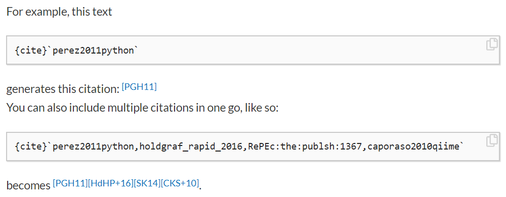
For example, here’s how you can include a citation in the new Jupyter Book:
A sample citation. Here we see how you can include citation syntax in-line with your markdown, and then insert a bibliography later on in your page. (source: https://executablebooks.org/)
A smarter build system
While the old version of Jupyter Book used a combination of Python and Jekyll to build your book’s HTML, the new Jupyter Book uses Python all the way through. This means that building the HTML for your book is as simple as:
jupyter-book build mybookname/
In addition, the new build system leverages Jupyter Cache to execute notebook content only if the code is updated, and to insert the outputs from the cache at build time. This saves you time by avoiding the need to re-execute code that hasn’t been changed.
An example build process. Here the jupyter-book command-line interface is used to convert a collection of content into an HTML book. (source: https://blog.jupyter.org/)
More book output types
By leveraging Sphinx, Jupyter Book will be able to support more complex outputs than just an HTML website. For example, we are currently prototyping PDF Outputs, both via HTML as well as via LaTeX. This gives Jupyter Book more flexibility to generate the right book for your use case.
You can also run Jupyter Book on individual pages. This means that you can write single-page content (like a scientific article) entirely in Markdown.
A new stack
The biggest change under-the-hood is that Jupyter Book now uses the Sphinx documentation engine instead of Jekyll for building books. By leveraging the Sphinx ecosystem, Jupyter Book can more effectively build on top of community tools, and can contribute components back to the broader community.
Instead of being a single repository, the old Jupyter Book repository has now been separated into several modular tools. Each of these tools can be used on their own in your Sphinx documentation, and they can be coordinated together via Jupyter Book:
MyST-NB is an .ipynb parser for Sphinx that allows you to use MyST Markdown in your notebooks. It also provides tools for execution, cacheing, and variable insertion of Jupyter Notebooks in Sphinx.
Jupyter Cache allows you to execute a collection of notebooks and store their outputs in a hashed database. This lets you cache your notebook’s output without including it in the .ipynb file itself.
Sphinx-Thebe converts your “static” HTML page into an interactive page with code cells that are run remotely by a Binder kernel.
Jupyter Book and its related projects will continue to be developed as a part of the Executable Book Project, a community that builds open source tools for high-quality scientific publications from computational content in the Jupyter ecosystem and beyond.
First off, make sure you have the CLI installed so that you can work with Jupyter Book. The Jupyter-Book CLI allows you to build and control your Jupyter Book. You can install it via pip with the following command:
pip install -U jupyter-book
The book building process
Building a Jupyter Book broadly consists of two steps:
Put your book content in a folder or a file. Jupyter Book needs the following pieces in order to build your book:
Your content file(s) (the pages of your book) in either markdown or Jupyter Notebooks.
A Table of Contents YAML file (_toc.yml) that defines the structure of your book. Mandatory when building a folder.
(optional) A configuration file (_config.yml) to control the behavior of Jupyter Book.
Build your book. Using Jupyter Book’s command-line interface you can convert your pages into either an HTML or a PDF book.
Host your book’s HTML online. Once your book’s HTML is built, you can host it online as a public website. See Publish your book online for more information.
Create a template Jupyter Book
We’ll use a small template book to show what kinds of files you might put inside your own. To create a new Jupyter Book, type the following at the command-line:
jupyter-book create mybookname
A new book will be created at the path that you’ve given (in this case, mybookname/).
If you would like to quickly generate a basic Table of Contents YAML file, run the following command:
jupyter-book toc mybookname/
And it will generate a TOC for you. Note that there must be at least one content file in each folder in order for any sub-folders to be parsed.
Inspecting your book’s contents
Let’s take a quick look at some important files in the demo book you created:
Here’s a quick rundown of the files you can modify for yourself, and that ultimately make up your book.
Book configuration
All of the configuration for your book is in the following file:
mybookname/
├── _config.yml
You can define metadata for your book (such as its title), add a book logo, turn on different “interactive” buttons (such as a Binder button for pages built from a Jupyter Notebook), and more.
Table of Contents
Jupyter Book uses your Table of Contents to define the structure of your book. For example, your chapters, sub-chapters, etc.
The Table of Contents lives at this location:
mybookname/
├── _toc.yml
This is a YAML file with a collection of pages, each one linking to a file in your content/ folder. Here’s an example of a few pages defined in toc.yml.
The top-most level of your TOC file are book chapters. Above, this is the “Features” page. Note that in this case the title of the page is not explicitly specified but is inferred from the source files. This behavior is controlled by the page_titles setting in _config.yml (see Files for more details). Each chapter can have several sections (defined in sections:) and each section can have several sub-sections. For more information about how section structure maps onto book structure, see How headers and sections map onto to book structure.
Each item in the _toc.yml file points to a single file. The links should be relative to your book’s folder and with no extension.
For example, in the example above there is a file in mybookname/content/notebooks.ipynb. The TOC entry that points to this file is here:
- file: features/notebooks
Book content
The markdown and ipynb files in your folder is your book’s content. Some content files for the demo book are shown below:
Note that the content files are either Jupyter Notebooks or Markdown files. These are the files that define “sections” in your book.
You can store these files in whatever collection of folders you’d like, note that the structure of your book when it is built will depend solely on the order of items in your _toc.yml file (see below section)
Book bibliography for citations
If you’d like to build a bibliography for your book, you can do so by including the following file:
mybookname/
└── references.bib
This BiBTex file can be used to insert citations into your book’s pages. For more information, see Citations and cross-references.
Next step: build your book
Now that you’ve got a Jupyter Book folder structure, we can create the HTML (or PDF) for each of your book’s pages.
Build your book
Once you’ve added content and configured your book, it’s time to build outputs for your book. We’ll use the jupyter-book build command-line tool for this.
Currently, there are two kinds of supported outputs: an HTML website for your book, and a PDF that contains all of the pages of your book that is built from the book HTML.
Prerequisites
In order to build the HTML for each page, you should have followed the steps in creating your Jupyter Book structure. You should have a collection of notebook/markdown files in your mybookname/ folder, a _toc.yml file that defines the structure of your book, and any configuration you’d like in the _config.yml file.
Build your book’s HTML
Now that your book’s content is in your book folder and you’ve defined your book’s structure in _toc.yml, you can build the HTML for your book.
Note: HTML is the default builder.
Do so by running the following command:
jupyter-book build mybookname/
This will generate a fully-functioning HTML site using a static site generator. The site will be placed in the _build/html folder. You can then open the pages in the site by entering that folder and opening the html files with your web browser.
Note: You can also use the short-hand jb for jupyter-book. E.g.,: jb build mybookname/.
Build a standalone page
Sometimes you’d like to build a single page of content rather than an entire book. For example, if you’d like to generate a web-friendly HTML page from a Jupyter Notebook for a report or publication.
You can generate a standalone HTML file for a single page of the Jupyter Book using the same command :
jupyter-book build path/to/mypage.ipynb
This will execute your content and output the proper HTML in a _build/html folder.
Your page will be called mypage.html. This will work for any content source file that is supported by Jupyter Book.
Note: Users should note that building single pages in the context of a larger project, can trigger warnings and incomplete links. For example, building docs/start/overview.md will issue a bunch of unknown document,term not in glossary, and undefined links warnings.
Page caching
By default, Jupyter Book will only build the HTML for pages that have been updated since the last time you built the book. This helps reduce the amount of unnecessary time needed to build your book. If you’d like to force Jupyter Book to re-build a particular page, you can either edit the corresponding file in your book’s folder, or delete that page’s HTML in the _build/html folder.
Local preview
To preview your book, you can open the generated HTML files in your browser. Either double-click the html file in your local folder, or enter the absolute path to the file in your browser navigation bar adding file:// at the beginning (e.g. file://Users/my_path_to_book/_build/index.html).
Next step: publish your book
Now that you’ve created the HTML for your book, it’s time to publish it online.
Publish your book online
Once you’ve built the HTML for your book, you can host it online. The best way to do this is with a service that hosts static websites (because that’s what you have just created with Jupyter Book). There are many options for doing this, and these sections cover some of the more popular ones.
Create an online repository for your book
Regardless of the approach you use for publishing your book online, it will require you to host your book’s content in an online repository such as GitHub. This section describes one approach you can use to create your own GitHub repository and add your book’s content to it.
First, log-in to GitHub, then go to the “create a new repository” page:https://github.com/new
Next, give your online repository a name and a description. Make your repository public and do not initialize with a README file, then click “Create repository”.
Now, clone the (currently empty) online repository to a location on your local computer. You can do this via the command line with:
4. Copy all of your book files and folders into this newly cloned repository. For example, if you created your book locally with jupyter-book create mylocalbook and your new repository is called myonlinebook, you could do this via the command line with:
cp -r mylocalbook/* myonlinebook/
5. Now you need to sync your local and remote (i.e., online) repositories. You can do this with the following commands:
cd myonlinebook
git add ./*
git commit -m "adding my first book!"
git push
Thanks so much for your interest in my post!
If it was useful for you, please remember to “Clap” 👏 it so other people can also benefit from it.
If you have any suggestions or questions, please leave a comment!
Reimagining what a Jupyter notebook can be and what can be done with it.
Netflix aims to provide personalized content to their 130 million viewers. One of the significant ways by which data scientists and engineers at Netflix interact with their data is through Jupyter notebooks. Notebooks leverage the use of collaborative, extensible, scalable, and reproducible data science. For many of us, Jupyter Notebooks is the de facto platform when it comes to quick prototyping and exploratory analysis. However, there’s more to this than meets the eye. A lot of Jupyter functionalities sometimes lies under the hood and is not adequately explored. Let us try and explore Jupyter Notebooks’ features which can enhance our productivity while working with them.
Table of Contents
Executing Shell Commands
Jupyter Themes
Notebook Extensions
Jupyter Widgets
Qgrid
Slideshow
Embedding URLs, PDFs, and Youtube Videos
1. Executing Shell Commands
The notebook is the new shell
The shell is a way to interact textually with the computer. The most popular Unix shell is Bash(Bourne Again SHell ). Bash is the default shell on most modern implementations of Unix and in most packages that provide Unix-like tools for Windows.
Now, when we work with any Python interpreter, we need to regularly switch between the shell and the IDLE, in case we need to use the command line tools. However, the Jupyter Notebook gives us the ease to execute shell commands from within the notebook by placing an extra !before the commands. Any command that works at the command-line can be used in IPython by prefixing it with the ! character.
In [1]: !ls
example.jpeg list tmpIn [2]: !pwd
/home/Parul/Desktop/Hello World Folder'In [3]: !echo "Hello World"
Hello World
We can even pass values to and from the shell as follows:
Notice, the data type of the returned results is not a list.
2. Jupyter Themes
Theme-ify your Jupyter Notebooks!
If you are a person who gets bored while staring at the white background of the Jupyter notebook, themes are just for you. The themes also enhance the presentation of the code. You can find more about Jupyter themes here. Let’s get to the working part.
Installation
pip install jupyterthemes
List of available themes
jt -l
Currently, the available themes are chesterish, grade3, gruvboxd, gruvboxl monokai, oceans16, onedork, solarizedd ,solarizedl.
# selecting a particular themejt -t <name of the theme># reverting to original Themejt -r
You will have to reload the jupyter notebook everytime you change the theme, to see the effect take place.
The same commands can also be run from within the Jupyter Notebook by placing ‘!’ before the command.
Left: original | Middle: Chesterish Theme | Right: solarizedl theme
3. Notebook Extensions
Extend the possibilities
Notebook extensions let you move beyond the general vanilla way of using the Jupyter Notebooks. Notebook extensions (or nbextensions) are JavaScript modules that you can load on most of the views in your Notebook’s frontend. These extensions modify the user experience and interface.
pip install jupyter_contrib_nbextensions && jupyter contrib nbextension install#incase you get permission errors on MacOS,pip install jupyter_contrib_nbextensions && jupyter contrib nbextension install --user
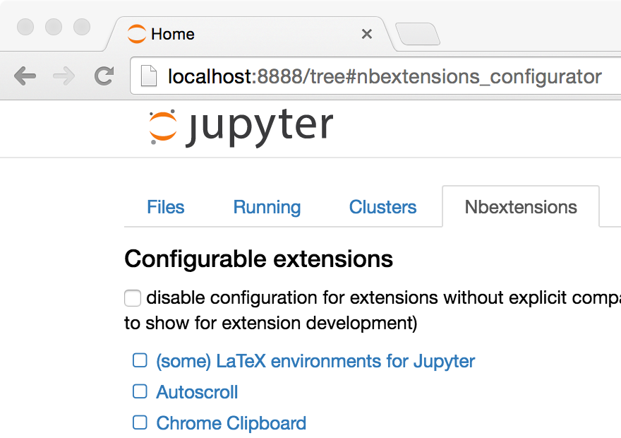
Start a Jupyter notebook now, and you should be able to see an NBextensions Tab with a lot of options. Click the ones you want and see the magic happen.
In case you couldn’t find the tab, a second small nbextension, can be located under the menuEdit.
Let us discuss some of the useful extensions.
1. Hinterland
Hinterland enables code autocompletion menu for every keypress in a code cell, instead of only calling it with the tab. This makes Jupyter notebook’s autocompletion behave like other popular IDEs such as PyCharm.
2. Snippets
This extension adds a drop-down menu to the Notebook toolbar that allows easy insertion of code snippet cells into the current notebook.
3. Split Cells Notebook
This extension splits the cells of the notebook and places then adjacent to each other.
4. Table of Contents
This extension enables to collect all running headers and display them in a floating window, as a sidebar or with a navigation menu. The extension is also draggable, resizable, collapsible and dockable.
5. Collapsible Headings
Collapsible Headings allows the notebook to have collapsible sections, separated by headings. So in case you have a lot of dirty code in your notebook, you can simply collapse it to avoid scrolling it again and again.
6. Autopep8
Autopep8 helps to reformat/prettify the contents of code cells with just a click. If you are tired of hitting the spacebar again and again to format the code, autopep8 is your savior.
4. Jupyter Widgets
Make notebooks interactive
Widgets are eventful python objects that have a representation in the browser, often as a control like a slider, textbox, etc. Widgets can be used to build interactive GUIs for the notebooks.
Let us have a look at some of the widgets. For complete details, you can visit their Github repository.
Interact
The interact function (ipywidgets.interact) automatically creates a user interface (UI) controls for exploring code and data interactively. It is the easiest way to get started using IPython's widgets.
# Start with some imports!from ipywidgets import interact
import ipywidgets as widgets
1. Basic Widgets
def f(x):
    return x# Generate a slider
interact(f, x=10,);
The Play widget is useful to perform animations by iterating on a sequence of integers at a certain speed. The value of the slider below is linked to the player.
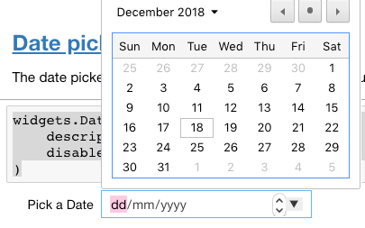
The date picker widget works in Chrome and IE Edge but does not currently work in Firefox or Safari because they do not support the HTML date input field.
widgets.DatePicker(
    description='Pick a Date',
    disabled=False
)
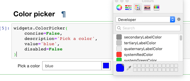
Color picker
widgets.ColorPicker(
    concise=False,
    description='Pick a color',
    value='blue',
    disabled=False
)
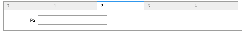
tab_contents = ['P0', 'P1', 'P2', 'P3', 'P4']
children = [widgets.Text(description=name) for name in tab_contents]
tab = widgets.Tab()
tab.children = children
for i in range(len(children)):
    tab.set_title(i, str(i))
tab
5. Qgrid
Make Data frames intuitive
Qgrid is also a Jupyter notebook widget but mainly focussed at dataframes. It uses SlickGrid to render pandas DataFrames within a Jupyter notebook. This allows you to explore your DataFrames with intuitive scrolling, sorting and filtering controls, as well as edit your DataFrames by double-clicking cells. The Github Repository contains more details and examples.
Installation
Installing with pip:
pip install qgrid
jupyter nbextension enable --py --sys-prefix qgrid# only required if you have not enabled the ipywidgets nbextension yet
jupyter nbextension enable --py --sys-prefix widgetsnbextension
Installing with conda:
# only required if you have not added conda-forge to your channels yet
conda config --add channels conda-forgeconda install qgrid
6. Slideshow
Code is great when communicated.
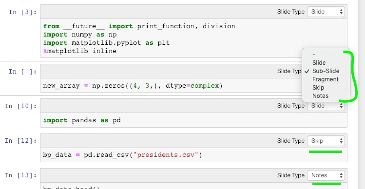
Notebooks are an effective tool for teaching and writing explainable codes. However, when we want to present our work either we display our entire notebook(with all the codes) or we take the help of powerpoint. Not any more. Jupyter Notebooks can be easily converted to slides and we can easily choose what to show and what to hide from the notebooks.
There are two ways to convert the notebooks into slides:
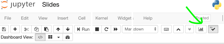
1. Jupyter Notebook’s built-in Slide option
Open a new notebook and navigate to View → Cell Toolbar → Slideshow. A light grey bar appears on top of each cell, and you can customize the slides.
Now go to the directory where the notebook is present and enter the following code:
jupyter nbconvert *.ipynb --to slides --post serve
# insert your notebook name instead of *.ipynb
The slides get displayed at port 8000. Also, a .html file will be generated in the directory, and you can also access the slides from there.
This would look even more classy with a themed background. Let us apply the theme ’onedork’ to the notebook and then convert it into a slideshow.
These slides have a drawback i.e. you can see the code but cannot edit it. RISE plugin offers a solution.
2. Using the RISE plugin
RISE is an acronym for Reveal.js — Jupyter/IPython Slideshow Extension. It utilized the reveal.js to run the slideshow. This is super useful since it also gives the ability to run the code without having to exit the slideshow.
Installation
1 — Using conda (recommended):
conda install -c damianavila82 rise
2 — Using pip (less recommended):
pip install RISE
and then two more steps to install the JS and CSS in the proper places:
Let us now use RISE for the interactive slideshow. We shall re-open the Jupyter Notebook we created earlier. Now we notice a new extension that says “Enter/Exit RISE Slideshow.”
Click on it, and you are good to go. Welcome to the world of interactive slides.
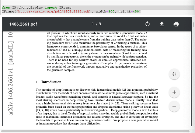
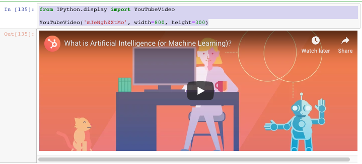
Why go with mere links when you can easily embed an URL, pdf, and videos into your Jupyter Notebooks using IPython’s display module.
URLs
#Note that http urls will not be displayed. Only https are allowed inside the Iframefrom IPython.display import IFrame
IFrame('https://en.wikipedia.org/wiki/HTTPS', width=800, height=450)
from IPython.display import YouTubeVideoYouTubeVideo('mJeNghZXtMo', width=800, height=300)
Conclusion
These were some of the features of the Jupyter Notebooks that I found useful and worth sharing. Some of them would be obvious to you while some may be new. So, go ahead and experiment with them. Hopefully, they will be able to save you some time and give you a better UI experience. Also feel free to suggest other useful features in the comments.
As someone who did over a decade of development before moving into Data Science, there’s a lot of mistakes I see data scientists make while using Pandas. The good news is these are really easy to avoid, and fixing them can also make your code more readable.
It’s nobody’s fault that there are way too many ways to get and set values in Pandas. In some situations, you have to find a value using only an index or find the index using only the value. However, in many cases, you’ll have many different ways of selecting data at your disposal: index, value, label, etc.
In those situations, I prefer to use whatever is fastest. Here are some common choices from slowest to fastest, which shows you could be missing out on a 195% gain!
Tests were run using a DataFrame of 20,000 rows. Here’s the notebook if you want to run it yourself.
# .at - 22.3 seconds
for i in range(df_size):
    df.at[i] = profile
Wall time: 22.3 s# .iloc - 15% faster than .at
for i in range(df_size):
    df.iloc[i] = profile
Wall time: 19.1 s# .loc - 30% faster than .at
for i in range(df_size):
    df.loc[i] = profile
Wall time: 16.5 s# .iat, doesn't work for replacing multiple columns of data.
# Fast but isn't comparable since I'm only replacing one column.
for i in range(df_size):
    df.iloc[i].iat[0] = profile['address']
Wall time: 3.46 s# .values / .to_numpy() - 195% faster than .at
for i in range(df_size):
    df.values[i] = profile
    # Recommend using to_numpy() instead if you have Pandas 1.0+
    # df.to_numpy()[i] = profile
Wall time: 254 ms
(As Alex Bruening and miraculixxnoted in the comments, for loops are not the ideal way to perform actions like this, look at .apply(). I’m using them here purely to prove the speed difference of the line inside the loop.)
Mistake 2: Only Using 25% of Your CPU
Whether you’re on a server or just your laptop, the vast majority of people never use all the computing power they have. Most processors (CPUs) have 4 cores nowadays, and by default, Pandas will only ever use one.
From the Modin Docs, a 4x speedup on a 4 core machine.
Modin is a Python module built to enhance Pandas by making way better use of your hardware. Modin DataFrames don’t require any extra code and in most cases will speed up everything you do to DataFrames by 3x or more.
Modin acts as more of a plugin than a library since it uses Pandas as a fallback and cannot be used on its own.
The goal of Modin is to augment Pandas quietly and let you keep working without learning a new library. The only line of code most people will need is import modin.pandas as pd replacing your normal import pandas as pd, but if you want to learn more check out the documentation here.
In order to avoid recreating tests that have already been done, I’ve included this picture from the Modin documentation showing how much it can speed up the read_csv() function on a standard laptop.
Please note that Modin is in development, and while I use it in production, you should expect some bugs. Check the Issues in GitHub and the Supported APIs for more information.
Mistake 3: Making Pandas Guess Data Types
When you import data into a DataFrame and don’t specifically tell Pandas the columns and datatypes, Pandas will read the entire dataset into memory just to figure out the data types.
For example, if you have a column full of text Pandas will read every value, see that they’re all strings, and set the data type to “string” for that column. Then it repeats this process for all your other columns.
You can use df.info() to see how much memory a DataFrame uses, that’s roughly the same amount of memory Pandas will consume just to figure out the data types of each column.
Unless you’re tossing around tiny datasets or your columns are changing constantly, you should always specify the data types. In order to do this, just add the dtypes parameter and a dictionary with your column names and their data types as strings. For example:
Note: This also applies to DataFrames that don’t come from CSVs.
Mistake 4: Leftover DataFrames
One of the best qualities of DataFrames is how easy they are to create and change. The unfortunate side effect of this is most people end up with code like this:
# Change dataframe 1 and save it into a new dataframedf1 = pd.read_csv(‘file.csv’)df2 = df1.dropna()df3 = df2.groupby(‘thing’)
What happens is you leave df2 and df1 in Python memory, even though you’ve moved on to df3. Don’t leave extra DataFrames sitting around in memory, if you’re using a laptop it’s hurting the performance of almost everything you do. If you’re on a server, it’s hurting the performance of everyone else on that server (or at some point, you’ll get an “out of memory” error).
Instead, here are some easy ways to keep your memory clean:
Use df.info() to see how much memory a DataFrame is using
If you’re in a Jupyter session already, you can always erase variables without restarting by using del df2
Chain together multiple DataFrame modifications in one line (so long as it doesn’t make your code unreadable): df = df.apply(thing1).dropna()
As Roberto Bruno Martins pointed out, another way to ensure clean memory is to perform operations within functions. You can still unintentionally abuse memory this way, and explaining scope is outside the scope of this article, but if you aren’t familiar I’d encourage you to read this writeup.
Mistake 5: Manually Configuring Matplotlib
This might be the most common mistake, but it lands at #5 because it’s the least impactful. I see this mistake happen even in tutorials and blog posts from experienced professionals.
Matplotlib is automatically imported by Pandas, and it even sets some chart configuration up for you on every DataFrame.
There’s no need to import and configure it for every chart when it’s already baked into Pandas for you.
Here’s an example of doing it the wrong way, even though this is a basic chart it’s still a waste of code:
import matplotlib.pyplot as plt
ax.hist(x=df[‘x’])
ax.set_xlabel(‘label for column X’)
plt.show()
I’m sure I’m making other mistakes I don’t know about, but hopefully sharing these known ones with you will help put your hardware to better use, let you write less code, and get more done!
If you’re still looking for more optimizations, you’ll definitely want to read:
ipywidgets plays an essential part in the Jupyter ecosystem; it brings interactivity between user and data.
Widgets are eventful Python objects that often have a visual representation in the Jupyter Notebook or JupyterLab: a button, a slider, a text input, a checkbox…
More than a library of interactive widgets, ipywidgetsis a powerful framework upon which it is straightforward to create new custom widgets. Developers can quickly start their own widgets library with best practices of code structure and packaging using the widget-cookiecutterproject.
A spreadsheet is an interactive tool for data analysis in a tabular form. It consists of cells and cell ranges. It supports value dependent cell formatting/styling and one can apply mathematical functions on cells and perform chained computations. It is the perfect user interface for statistical and financial operations.
The Jupyter Notebook was lacking a spreadsheet library, that’s when ipysheet comes into play.
ipysheet
ipysheet is a new interactive widgets library that aims at implementing the core features of a good spreadsheet application and more.
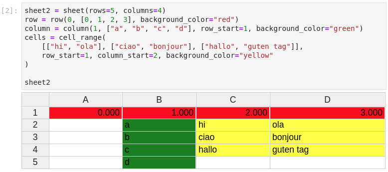
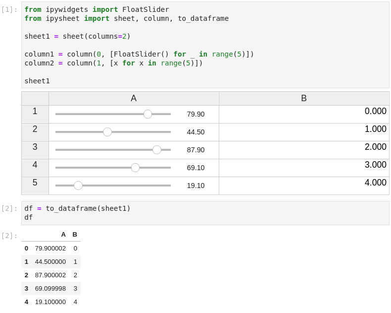
There are two main widgets in ipysheet, the Cell widget, and the Sheet widget. We provide helper functions for creating rows, columns and cell ranges in general.
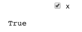
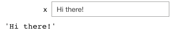
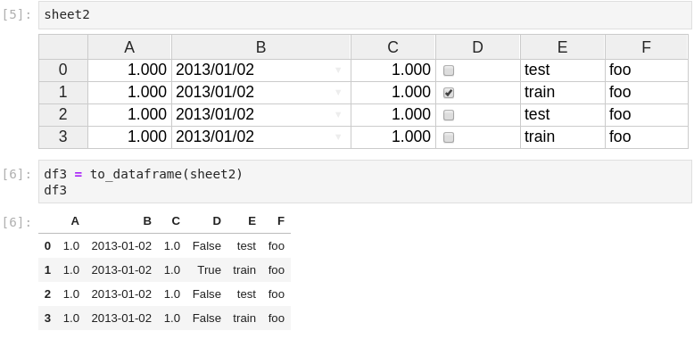
The cell value can be a boolean, a numerical value, a string, a date, and of course another widget!
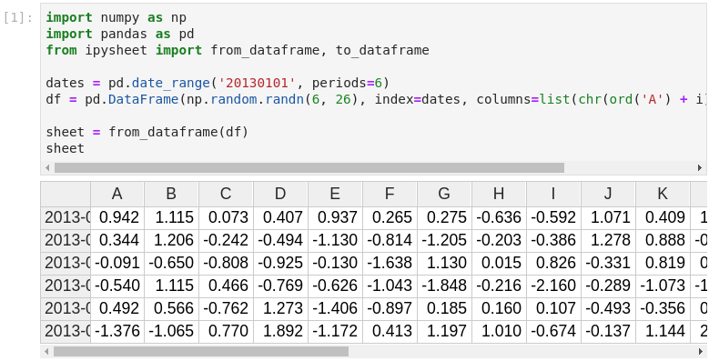
ipysheetuses a Matplotlib-like API for creating a sheet:
The user can create entire rows, columns, and even cell ranges:
Of course, values in cells are dynamic, the cell value can be dynamically updated from Python and the new value will be visible in the sheet.
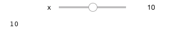
It is possible to link a cell value to a widget (in the following screenshot a FloatSlider widget is linked to cell “a”) and to define a specific cell as the result of a custom calculation depending on other cells:
Custom styling can be used, using what we call renderers:
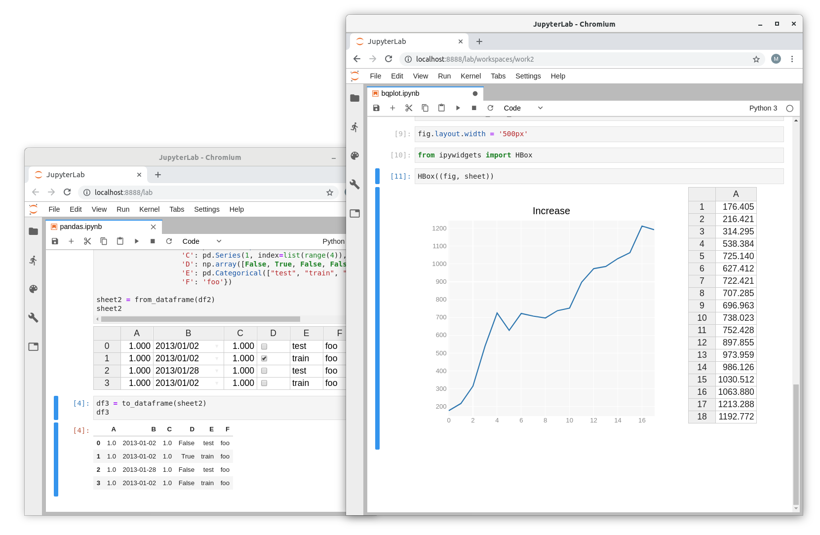
Adding support to NumPy Arrays and Pandas Dataframes loading and exporting was an important feature that we wanted. ipysheetprovides from_array, to_array, from_dataframe and to_dataframe functions for this purpose:
Another killer feature is that a cell value can be ANY interactive widget. This means that the user can put a button or a slider widget in a cell:
But it also means that a higher level widget can be put in a cell. Whether the widget is a plot from bqplot, a map from ipyleaflet or even a multi-volume rendering from ipyvolume:
You can try it right now with binder, without the need of installing anything on your computer, just by clicking on this button:
This development is sponsored by Société Générale and Bloomberg.
About the Authors
Maarten Breddels is an entrepreneur and freelance developer / consultant / data scientist working mostly with Python, C++ and Javascript in the Jupyter ecosystem. Founder of vaex.io. His expertise ranges from fast numerical computation, API design, to 3d visualization. He has a Bachelor in ICT, a Master and PhD in Astronomy, likes to code and solve problems.
Martin Renou is a Scientific Software Engineer at QuantStack. Before joining QuantStack, he studied at the French Aerospace Engineering School SUPAERO. He also worked at Logilab in Paris and Enthought in Cambridge. As an open source developer at QuantStack, Martin worked on a variety of projects, from xsimd, xtensor, xframe, xeus and xeus-python in C++ to ipyleaflet and ipywebrtc in Python and JavaScript.