It’s ironic how developers use a plethora of apps and software to make…apps and software. Over time, we have developed strong preferences over a select few tools as part of their workflow. However, just because some pieces of software have become the norm that doesn’t mean we shouldn’t always be on the lookout for others! Here are some of the most underrated yet insanely useful apps that I’ve tried to use on a daily basis, and that I think you should use too!
Because I don’t want my recommendations to be focused towards a specific niche of programming, a noticeable fraction of apps shown below would be terminal-based, thus addressing the majority of programmers/developers.
Table of Contents
Ungit
Termius
Alacritty
Byobu
Spacedesk
1. Ungit
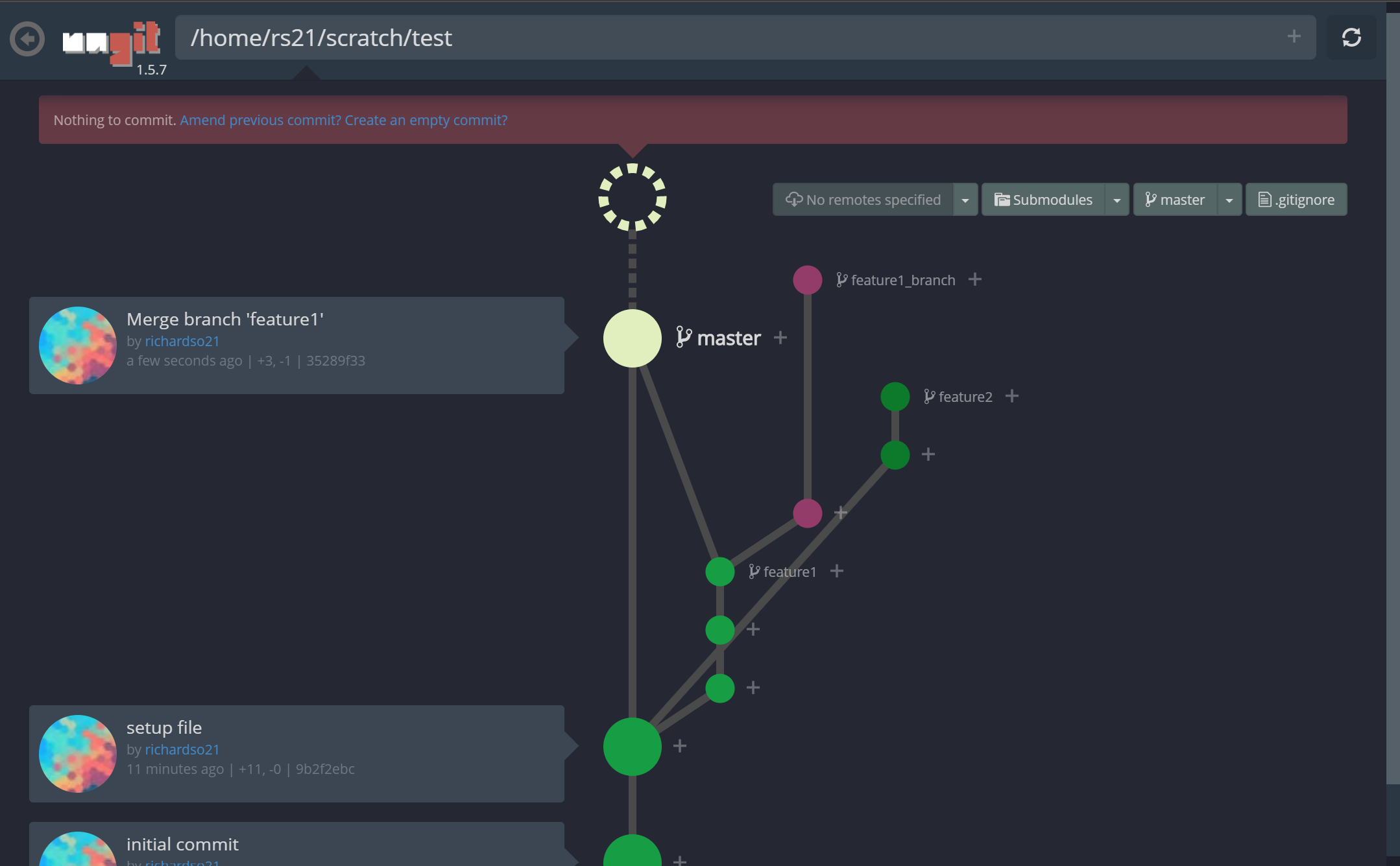
It is notoriously difficult to manage your Git repository through the command line interface — everyone knows that for a fact. And when you have a project open with 20 or so different branches, it’s hard to keep up with recent commits through all of them, let alone follow a branching model. Even worse are beginners trying to use Git for their first time to perform version control; a CLI can’t let users comprehend what Git really is supposed to be.
Ungit solves all of these issues with an intuitive GUI for managing Git repos.
Ungit represents your repo like a spider web of commits and branches. Here’s what it’ll look like in action:
A quick look into ungit
Look at those branches! Also, making commits are easier than ever, and paired with the fun animations, lets you feel a commit was done — something the command line can’t induce:
Creating a new commit in ungit
Checking out between branches is also relatively simple, and the UI lets you see the commit history relative to the branch you’re currently on:
Switching (Checking out) between different branches in the same repo in ungit
Ungit supports merging branches, tagging, and much more! You can find a more comprehensive demo on YouTube here.
2. Termius
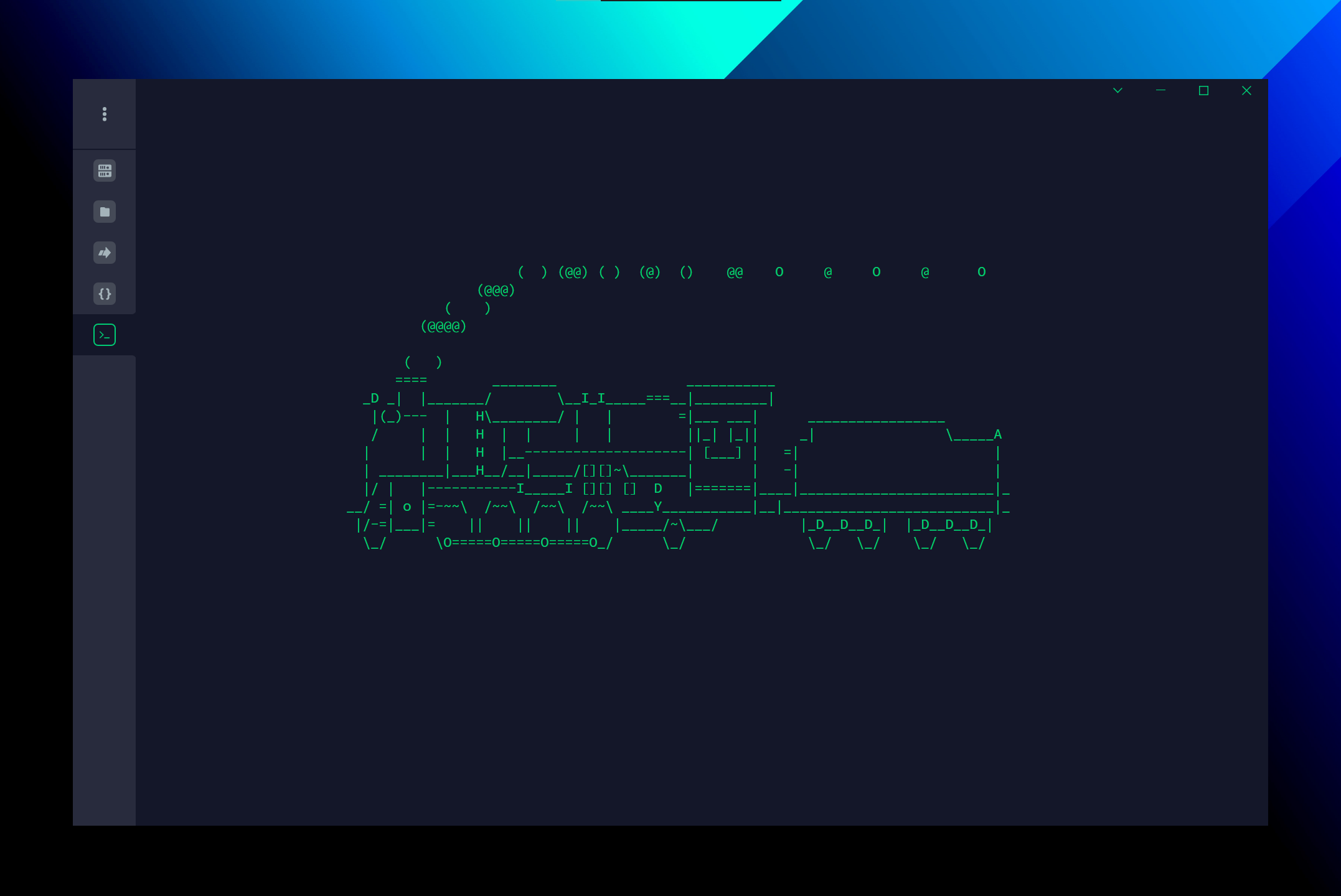
It’s quarantine time (at least at the time of writing this), so everybody is reasonably working from home. What if you need to access a computer or server at your workplace? Well, you would SSH into the server, giving yourself access to the terminal on that machine. Although this is doable with a simple ssh command, why not do it in style with Termius?
Termius is an Mosh-compatible SSH client, seemingly built on top of Electron (don’t quote me on that!), which works on all platforms you’d imagine — that’s Windows, macOS, Linux, iOS, and Android.
Running `sl`, on a remote server, on Termius 😎
Customization options for Termius
The app supports a plethora of themes, fonts, and font sizes, which you can customize to your liking. Not to mention, the app already looks pretty sleek with its default presets.
One of the most compelling features of Termius, apart from its looks and SSH capability, is port forwarding, which I frequently use for Jupyter.
It also supports remembering multiple hosts, which you can then sync with your mobile devices when you’re handling remote server processes on-the-go. Syncing is done through accounts, which you can sign up for free, or pay a little for extra added benefits.
3. Alacritty
Talking about terminals, Alacritty would be my go-to local terminal emulator. It is supported in Windows, macOS, and many linux distributions. One of the best selling points of Alacritty is its support for GPU acceleration. Because of this, the makers of the terminal emulator boast blazing fast performance compared to alternatives.
Alacritty comes in a much simpler package compared to Termius, however, that doesn’t mean that it lacks in customization. The app accepts a configuration file (in the form of an .ymlfile) that you can fiddle around, provided by their repo. There, you can customize practically anything about the terminal, from color schemes to keyboard bindings to even background opacity! Whether you are a terminal power user or just need it to access your local directories, try out Alacritty!
4. Byobu
This isn’t technically an app or piece of software, but I felt compelled to feature it in this article because I’ve personally used this so much in my workflow. It’s a terminal multiplexer & window manager— in fact, it’s actually a wrapper over tmux and/or GNU screen, which are multiplexers you might’ve heard of. If you’re either working on a remote server (on Termius 😉) or find yourself frequently opening multiple terminal windows on your own machine, Byobu is definitely for you.
Instead of opening multiple terminal instances, Byobu handles all terminal instances in one interface. Let’s say you have 2 terminals open for a task, and you need to easily access all of these at the same time. Let’s see this in action:
Using Byobu to handle terminal sessions/instances in one place
Fun fact: Byobu here is running under Alacritty!
As you can see, it’s extremely simple to create a new terminal instance and switch between the two. Your instances (or “windows” based on the documentation) are listed below at the status bar, which is already by itself filled with goodies, and this comes right out of the box!
Byobu’s defaultstatus bar
It doesn’t stop there: you can actually set up individual split panes in each window, letting you create the perfect terminal layout.
Splitting panes in Byobu
Byobu is, in my opinion, much easier to learn compared to other multiplexers out there. Byobu utilizes the function keys — like F1, F2, F3…etc. — for it’s main keyboard bindings. At least for me, putting everything on a row is a better idea than having it all over the place, even if some bindings might induce some hand cramps😅. And if you’re lost or a beginner, you can always press Shift+F1 to view a cheat sheet.
5. Spacedesk
I’ve made an article on this app recently over here. If you want more details of this, you can head on to that article as well!
Basically, Spacedesk lets you convert an iPad, old laptop with wifi, or even phone into a second monitor for your main machine. It might sound extremely niche right now, except when you realize how much time you spend just Alt-Tabbing everywhere.
So, instead of buying a second monitor or trying to make a DIY monitor out of spare parts, you can save time and money with this app. Personally, I’ve used this to revive my old laptop with a new purpose, and I’ve seen little to no issues or bugs. The app runs completely wirelessly, so in exchange for better convenience and the lack of cables, your mileage may vary depending on how good your internet connection is.
Spacedesk is still in its beta stage, however, it plans to make it’s first release version later this year, so stay tuned!
Conclusion
That’s about it for some underrated apps/software you should start using today! If you have thoughts or some alternatives to ones I’ve listed feel free to let me know and start a conversation below. As always, happy coding, everybody!
Python is one of the most popular languages used by many in data science and machine learning, web development, scripting, automation, and more. One of the reasons for this popularity is its simplicity and ease of learning.
If you are reading this, you are most likely already using Python, or at least interested in it.
In this article, we’ll take a quick look at 29 short code snippets that you can understand and master incredibly quickly. Go!
👉 1. Checking for uniqueness
The next method checks if there are duplicate items in the given list. It uses a property set()that removes duplicate items from the list:
👉 2. Anagram
This method can be used to check if two strings are anagrams. An Anagram is a word or phrase formed by rearranging the letters of another word or phrase, usually using all the original letters exactly once:
👉 3. Memory
And this can be used to check the memory usage of an object:
👉 4. Size in bytes
The method returns the length of the string in bytes:
👉 5. Print the string N times
This snippet can be used to output a string nonce without the need to use loops for this:
👉 6. Makes the first letters of words large
And here is the register. The snippet uses a method title()to capitalize each word in a string:
👉 7. Separation
This method splits the list into smaller lists of the specified size:
👉 8. Removing false values
So you remove the false values ( False, None, 0and «») from the list using filter():
👉 9. Counting
The following code can be used to transpose a 2D array:
👉 10. Chain comparison
You can do multiple comparisons with all kinds of operators in one line:
👉 11. Separate with comma
The following snippet can be used to convert a list of strings to a single string, where each item from the list is separated by commas:
👉 12. Count the vowels
This method counts the number of vowels (“a”, “e”, “i”, “o”, “u”) found in the string:
👉 13. Converting the first letter of a string to lowercase
Use to convert the first letter of your specified string to lowercase:
👉 14. Anti-aliasing
The following methods flatten out a potentially deep list using recursion:
👉 15. Difference
The method finds the difference between the two iterations, keeping only the values that are in the first:
👉 16. The difference between lists
The following method returns the difference between the two lists after applying this function to each element of both lists:
👉 17. Chained function call
You can call multiple functions on one line:
👉 18. Finding Duplicates
This code checks to see if there are duplicate values in the list using the fact that set()it only contains unique values:
👉 19. Combine two dictionaries
The following method can be used to combine two dictionaries:
👉 20. Convert two lists to a dictionary
Now let’s get down to converting two lists into a dictionary:
👉 21. Using `enumerate`
The snippet shows what you can use enumerate()to get both values and indices of lists:
👉 22. Time spent
Use to calculate the time it takes for a specific code to run:
👉 23. Try / else
You can use elseas part of a block try:
👉 24. The element that appears most often
This method returns the most frequent item that appears in the list:
👉 25. Palindrome
The method checks if the given string is a palindrome:
👉 26. Calculator without if-else
The following snippet shows how to write a simple calculator without the need for conditions if-else:
👉 27. Shuffle
This code can be used to randomize the order of items in a list. Note that shuffleworks in place and returns None:
👉 28. Change values
A really quick way to swap two variables without the need for an extra one:
👉 29. Get default value for missing keys
The code shows how you can get the default value if the key you are looking for is not included in the dictionary:
Read More
If you found this article helpful, click the💚 or 👏 button below or share the article on Facebook so your friends can benefit from it too.
A few days ago when I browsed the “learnpython” sub on Reddit, I saw a Redditor asking this question again. Although there are too many answers and explanations about this question on the Internet, many beginners still do not know about it and make mistakes. Here is the question
Both “==” and “is” are operators in Python(Link to operator page in Python). For beginners, they may interpret “a == b” as “a is equal to b” and “a is b” as, well, “a is b”. Probably this is the reason why beginners confuse “==” and “is” in Python.
I want to show some examples of using “==” and “is” first before the in-depth discussion.
>>> a = 5
>>> b = 5
>>> a == b
True
>>> a is b
True
Simple, right? a == b and a is b both return True. Then go to the next example.
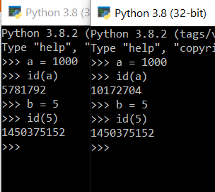
>>> a = 1000
>>> b = 1000
>>> a == b
True
>>> a is b
False
WTF ?!? The only change from the first example to the second is the values of a and b from 5 to 1000. But the results already differ between “==” and “is”. Go to the next one.
>>> a = []
>>> b = []
>>> a == b
True
>>> a is b
False
Here is the last example if your mind is still not blown.
>>> a = 1000
>>> b = 1000
>>> a == b
True
>>> a is b
False
>>> a = b
>>> a == b
True
>>> a is b
True
The official operation for “==” is equality while the operation for “is” is identity. You use “==” for comparing the values of two objects. “a == b” should be interpreted as “The value of a is whether equal to the value of b”. In all examples above, the value of a is always equal to the value of b (even for the empty list example). Therefore “a == b” is always true.
Before explaining identity, I need to first introduce id function. You can get the identity of an object with idfunction. This identity is unique and constant for this object throughout the time. You can think of this as an address for this object. If two objects have the same identity, their values must be also the same.
>>> id(a)
2047616
The operator “is” is to compare whether the identities of two objects are the same. “a is b” means “The identity of a is the same as the identity of b”.
Once you know the actual meanings of “==” and “is”, we can start going deep on those examples above.
First is the different results in the first and second examples. The reason for showing different results is that Python stores an array list of integers from -5 to 256 with a fixed identity for each integer. When you assign a variable of an integer within this range, Python will assign the identity of this variable as the one for the integer inside the array list. As a result, for the first example, since the identities of a and b are both obtained from the array list, their identities are of course the same and therefore a is bis True.
>>> a = 5
>>> id(a)
1450375152
>>> b = 5
>>> id(b)
1450375152
But once the value of this variable falls outside this range, since Python inside does not have an object with that value, therefore Python will create a new identity for this variable and assign the value to this variable. As said before, the identity is unique for each creation, therefore even the values of two variables are the same, their identities are never equal. That’s why a is bin the second example is False
>>> a = 1000
>>> id(a)
12728608
>>> b = 1000
>>> id(b)
13620208
(Extra: if you open two consoles, you will get the same identity if the value is still within the range. But of course, this is not the case if the value falls outside the range.)
Once you understand the difference between the first and second examples, it is easy to understand the result for the third example. Because Python does not store the “empty list” object, so Python creates one new object and assign the value “empty list”. The result will be the same no matter the two lists are empty or with identical elements.
>>> a = [1,10,100,1000]
>>> b = [1,10,100,1000]
>>> a == b
True
>>> a is b
False
>>> id(a)
12578024
>>> id(b)
12578056
Finally, we move on to the last example. The only difference between the second and the last example is that there is one more line of code a = b.However this line of code changes the destiny of the variable a. The below result tells you why.
>>> a = 1000
>>> b = 2000
>>> id(a)
2047616
>>> id(b)
5034992
>>> a = b
>>> id(a)
5034992
>>> id(b)
5034992
>>> a
2000
>>> b
2000
As you can see, after a = b, the identity of a changes to the identity of b. a = bassigns the identity of bto a. So both aand b have the same identity, and thus the value of a now is the same as the value of b, which is 2000.
The last example tells you an important message that you may accidentally change the value of an object without notice, especially when the object is a list.
>>> a = [1,2,3]
>>> id(a)
5237992
>>> b = a
>>> id(b)
5237992
>>> a.append(4)
>>> a
[1, 2, 3, 4]
>>> b
[1, 2, 3, 4]
From the above example, because both a and bhave the same identity, their values must be the same. And thus after appending a new element to a, the value of bwill be also impacted. To prevent this situation, if you want to copy the value from one object to another object without referring to the same identity, the one for all method is to use deepcopyin the module copy (Link to Python document). For list, you can also perform by b = a[:] .
Scikit-learn (sklearn) is a powerful open source machine learning library built on top of the Python programming language. This library contains a lot of efficient tools for machine learning and statistical modeling, including various classification, regression, and clustering algorithms.
In this article, I will show 6 tricks regarding the scikit-learn library to make certain programming practices a bit easier.
1. Generate random dummy data
To generate random ‘dummy’ data, we can make use of the make_classification() function in case of classification data, and make_regression() function in case of regression data. This is very useful in some cases when debugging or when you want to try out certain things on a (small) random data set.
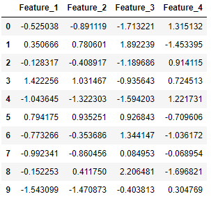
Below, we generate 10 classification data points consisting of 4 features (found in X) and a class label (found in y), where the data points belong to either the negative class (0) or the positive class (1):
from sklearn.datasets import make_classification
import pandas as pdX, y = make_classification(n_samples=10, n_features=4, n_classes=2, random_state=123)
Here, X consists of the 4 feature columns for the generated data points:
And y contains the corresponding label of each data point:
pd.DataFrame(y, columns=['Label'])
2. Impute missing values
Scikit-learn offers multiple ways to impute missing values. Here, we consider two approaches. The SimpleImputer class provides basic strategies for imputing missing values (through the mean or median for example). A more sophisticated approach the KNNImputer class, which provides imputation for filling in missing values using the K-Nearest Neighbors approach. Each missing value is imputed using values from the n_neighbors nearest neighbors that have a value for the particular feature. The values of the neighbors are averaged uniformly or weighted by distance to each neighbor.
Below, we show an example application using both imputation methods:
from sklearn.experimental import enable_iterative_imputer
from sklearn.impute import SimpleImputer, KNNImputer
from sklearn.datasets import make_classification
import pandas as pdX, y = make_classification(n_samples=5, n_features=4, n_classes=2, random_state=123)
X = pd.DataFrame(X, columns=['Feature_1', 'Feature_2', 'Feature_3', 'Feature_4'])print(X.iloc[1,2])
>>> 2.21298305
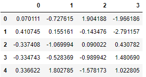
Transform X[1, 2] to a missing value:
X.iloc[1, 2] = float('NaN')X
First we make use of the simple imputer:
imputer_simple = SimpleImputer()

pd.DataFrame(imputer_simple.fit_transform(X))
Resulting in a value of -0.143476.
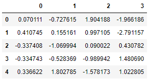
Next, we try the KNN imputer, where the 2 nearest neighbors are considered and the neighbors are weighted uniformly:
Resulting in a value of 0.997105 (= 0.5*(1.904188+0.090022)).
3. Make use of Pipelines to chain multiple steps together
The Pipeline tool in scikit-learn is very helpful to simplify your machine learning models. Pipelines can be used to chain multiple steps into one, so that the data will go through a fixed sequence of steps. Thus, instead of calling every step separately, the pipeline concatenates all steps into one system. To create such a pipeline, we make use of the make_pipeline function.
Below, a simple example is shown, where the pipeline consists of an imputer, which imputes missing values (if there are any), and a logistic regression classifier.
from sklearn.model_selection import train_test_split from sklearn.impute import SimpleImputer from sklearn.linear_model import LogisticRegression from sklearn.pipeline import make_pipeline from sklearn.datasets import make_classification import pandas as pdX, y = make_classification(n_samples=25, n_features=4, n_classes=2, random_state=123)
X_train, X_test, y_train, y_test = train_test_split(X, y, test_size=0.2, random_state=123)
Now, we can use the pipeline to fit our training data and to make predictions for the test data. First, the training data goes through to imputer, and then it starts training using the logistic regression classifier. Then, we are able to predict the classes for our test data:
Pipeline models created through scikit-learn can easily be saved by making use of joblib. In case your model contains large arrays of data, each array is stored in a separate file. Once saved locally, one can easily load (or, restore) their model for use in new applications.
from sklearn.model_selection import train_test_split from sklearn.impute import SimpleImputer from sklearn.linear_model import LogisticRegression from sklearn.pipeline import make_pipeline from sklearn.datasets import make_classification import joblibX, y = make_classification(n_samples=20, n_features=4, n_classes=2, random_state=123) X_train, X_test, y_train, y_test = train_test_split(X, y, test_size=0.2, random_state=123)
Now, the fitted pipeline model is saved (dumped) on your computer through joblib.dump. This model is restored through joblib.load, and can be applied as usual afterwards:
A confusion matrix is a table that is used to describe the performance of a classifier on a set of test data. Here, we focus on a binary classification problem, i.e., there are two possible classes that observations could belong to: “yes” (1) and “no” (0).
Let’s create an example binary classification problem, and display the corresponding confusion matrix, by making use of the plot_confusion_matrix function:
from sklearn.model_selection import train_test_split from sklearn.metrics import plot_confusion_matrix from sklearn.linear_model import LogisticRegression from sklearn.datasets import make_classificationX, y = make_classification(n_samples=1000, n_features=4, n_classes=2, random_state=123) X_train, X_test, y_train, y_test = train_test_split(X, y, test_size=0.2, random_state=123)
Here, we have visualized in a nice way through the confusion matrix that there are:
93 true positives (TP);
97 true negatives (TN);
3 false positives (FP);
7 false negatives (FN).
So, we have reached an accuracy score of (93+97)/200 = 95%.
6. Visualize decision trees
One of the most well known classification algorithms is the decision tree, characterized byits tree-like visualizations which are very intuitive. The idea of a decision tree is to split the data into smaller regions based on the descriptive features. Then, the most commonly occurring class amongst training observations in the region to which the test observation belongs is the prediction. To decide how the data is split into regions, one has to apply a splitting measure to determine the relevance and importance of each of the features. Some well known splitting measures are Information Gain, Gini index and Cross-entropy.
Below, we show an example on how to make use of the plot_tree function in scikit-learn:
from sklearn.model_selection import train_test_split from sklearn.tree import DecisionTreeClassifier, plot_tree from sklearn.datasets import make_classification
X, y = make_classification(n_samples=50, n_features=4, n_classes=2, random_state=123) X_train, X_test, y_train, y_test = train_test_split(X, y, test_size=0.2, random_state=123)
clf = DecisionTreeClassifier()
clf.fit(X_train, y_train)
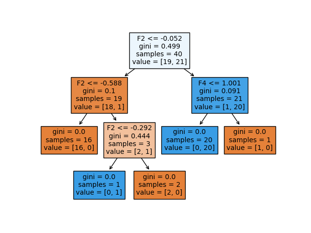
plot_tree(clf, filled=True)
In this example, we are fitting a decision tree on 40 training observations, that belong to either the negative class (0) or the positive class (1), so we are dealing with a binary classification problem. In the tree, we have two kinds of nodes, namely internal nodes (nodes where the predictor space is split further) or terminal nodes (end point). The segments of the trees that connect two nodes are called branches.
Let‘s have a closer look at the information provided for each node in the decision tree:
The splitting criterion used in the particular node is shown as e.g. ‘F2 <= -0.052’. This means that every data point that satisfies the condition that the value of the second feature is below -0.052 belongs to the newly formed region to the left, and the data points that do not satisfy the condition belong to the region to the right of the internal node.
The Gini index is used as splitting measure here. The Gini index (called a measure of impurity) measures the degree or probability of a particular element being wrongly classified when it is randomly chosen.
The ‘samples’ of the node indicates how many training observations are found in the particular node.
The ‘value’ of the node indicates the number of training observations found in the negative class (0) and the positive class (1) respectively. So, value=[19,21] means that 19 observations belong to the negative class and 21 observations belong to the positive class in that particular node.
Conclusion
This article covered 6 useful scikit-learn tricks to improve your machine learning models in sklearn. I hope these tricks have helped you in some way, and I wish you good luck on your next project when making use of the scikit-learn library!
Another cool behavior of the |= operator is the ability to update the dictionary with new key-value pairs using an iterable object — like a list or generator:
a = {'a': 'one', 'b': 'two'}
b = ((i, i**2) for i in range(3))a |= b
print(a)
[Out]: {'a': 'one', 'b': 'two', 0: 0, 1: 1, 2: 4}
If we attempt the same with the standard union operator | we will get a TypeError as it will only allow unions between dict types.
Type Hinting
Python is dynamically typed, meaning we don’t need to specify datatypes in our code.
This is okay, but sometimes it can be confusing, and suddenly Python’s flexibility becomes more of a nuisance than anything else.
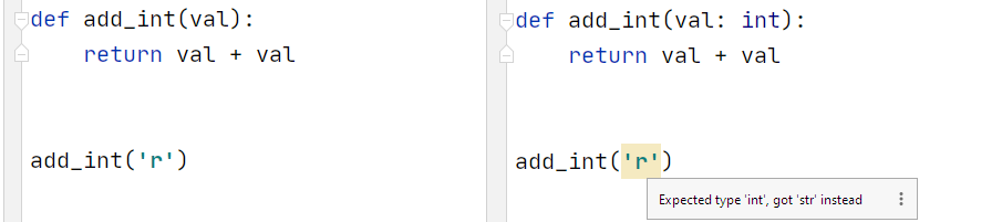
Since 3.5, we could specify types, but it was pretty cumbersome. This update has truly changed that, let’s use an example:
No type hinting (left) v type hinting with 3.9 (right)
In our add_int function, we clearly want to add the same number to itself (for some mysterious undefined reason). But our editor doesn’t know that, and it is perfectly okay to add two strings together using + — so no warning is given.
What we can now do is specify the expected input type as int. Using this, our editor picks up on the problem immediately.
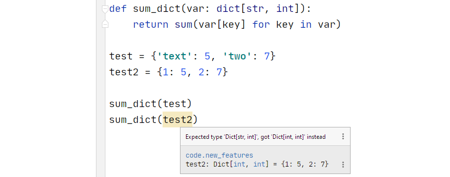
We can get pretty specific about the types included too, for example:
Type hinting can be used everywhere — and thanks to the new syntax, it now looks much cleaner:
We specify sum_dict’s argument as a dict and the returned value as an int. During test definition, we also determine it’s type.
String Methods
Not as glamourous as the other new features, but still worth a mention as it is particularly useful. Two new string methods for removing prefixes and suffixes have been added:
"Hello world".removeprefix("He")
[Out]: "llo world"
Hello world".removesuffix("ld")
[Out]: "Hello wor"
New Parser
This one is more of an out-of-sight change but has the potential of being one of the most significant changes for the future evolution of Python.
Python currently uses a predominantly LL(1)-based grammar, which in turn can be parsed by a LL(1) parser — which parses code top-down, left-to-right, with a lookahead of just one token.
Now, I have almost no idea of how this works — but I can give you a few of the current issues in Python due to the use of this method:
Python contains non-LL(1) grammar; because of this, some parts of the current grammar use workarounds, creating unnecessary complexity.
LL(1) creates limitations in the Python syntax (without possible workarounds). This issue highlights that the following code simply cannot be implemented using the current parser (raising a SyntaxError):
with (open("a_really_long_foo") as foo,
      open("a_really_long_bar") as bar):
    pass
LL(1) breaks with left-recursion in the parser. Meaning particular recursive syntax can cause an infinite loop in the parse tree. Guido van Rossum, the creator of Python, explains this here.
All of these factors (and many more that I simply cannot comprehend) have one major impact on Python; they limit the evolution of the language.
The new parser, based on PEG, will allow the Python developers significantly more flexibility — something we will begin to notice from Python 3.10 onwards.
That is everything we can look forward to with the upcoming Python 3.9. If you really can’t wait, the most recent beta release — 3.9.0b3 — is available here.
If you have any questions or suggestions, feel free to reach out via Twitter or in the comments below.
Thanks for reading!
If you enjoyed this article and want to learn more about some of the lesser-known features in Python, you may be interested in my previous article:
After completing the first module in my studies at Flatiron School NYC, I started playing with plot customizations and design using Seaborn and Matplotlib. Much like doodling during class, I started coding other styled plots in our jupyter notebooks.
After reading this article, you’re expected to have at least one quick styled plot code in mind for every notebook.
No more default, store brand, basic plots, please!
If you can do nothing else, use Seaborn.
You have five seconds to make a decent looking plot or the world will implode; use Seaborn!
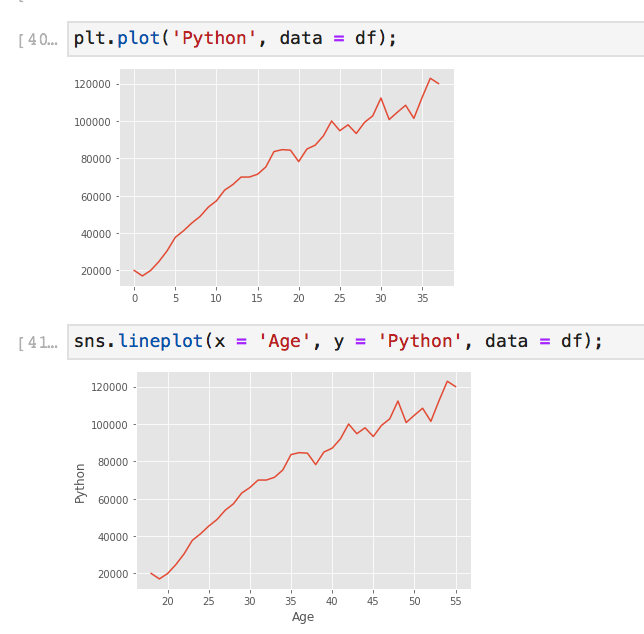
Seaborn, which is build using Matplotlib can be an instant design upgrade. It automatically assigns the labels from your x and y values and a default color scheme that’s less… basic. ( — IMO: it rewards good, clear, well formatted column labeling and through data cleaning) Matplotlib does not do this automatically, but also does not ask for x and y to be defined at all times depending on what you are looking to plot.
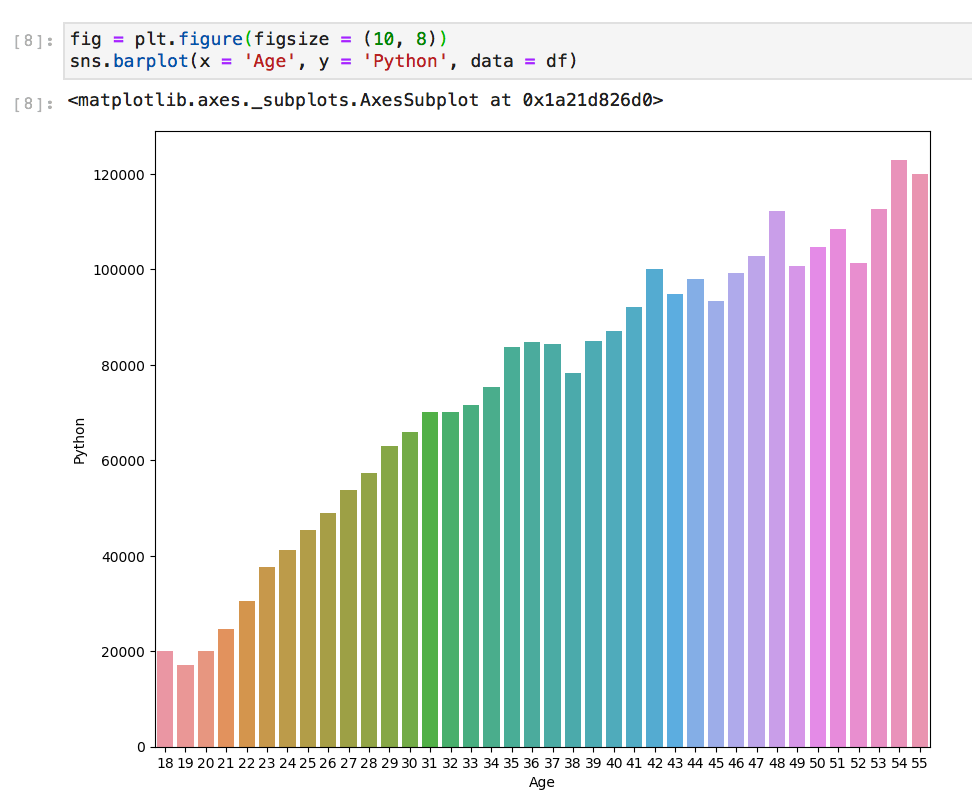
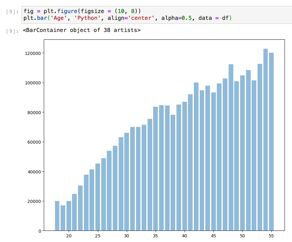
Here are the same plots, one using Seaborn and one Matplotlib with no customizations.
Depending on the data you are visualizing, changing the style and backgrounds may increase interpretability and readability. You can carry this style throughout by implementing a style at the top of your code.
There is a whole documentation page on styline via Matplotlib.
Styling can be as simple as setting the style with a simple line of code after your imported libraries. GGPlot changed the background to grey, and has a specific font. There are many more styles you can tryout.
Using plot styling, Matplotlib (top) Seaborn (bottom) Notice that Seaborn automatically labeled the plot.
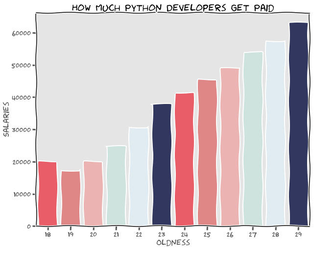
XKCD; a cheeky little extra
Fun. Not professional. But so fun.
Be aware that if you use this XKCD style it will continue until you reset the defaults by running plt.rcdefaults()…
PRETTY COLORS OMG!
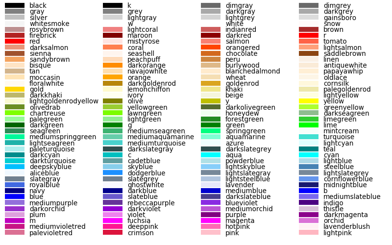
- Seaborn single color names. These can also be used in Matplot Lib. Image from Matplotlib.org
Make your plots engaging. Color theory comes into play here. Seaborn has a mix of palettes which can also be used in Matplot lib, plus you can also make your own.
Single Colors: One and Done
Above is a list of single color names you can call to change lines, scatter plots, and more.
Lazy? Seaborn’s Default Themes
has six variations of default
deep, muted, pastel, bright, dark, and colorblind
use color as an argument after passing in x, y, and data
color = ‘colorblind’
Work Smarter Not Harder: Pre-Fab Palettes
color_palette() accepts any seaborn palette or matplotlib colormap
create a kind and add in specifics, play around with the parameters for more customized palettes
Many ways to choose a color palette.
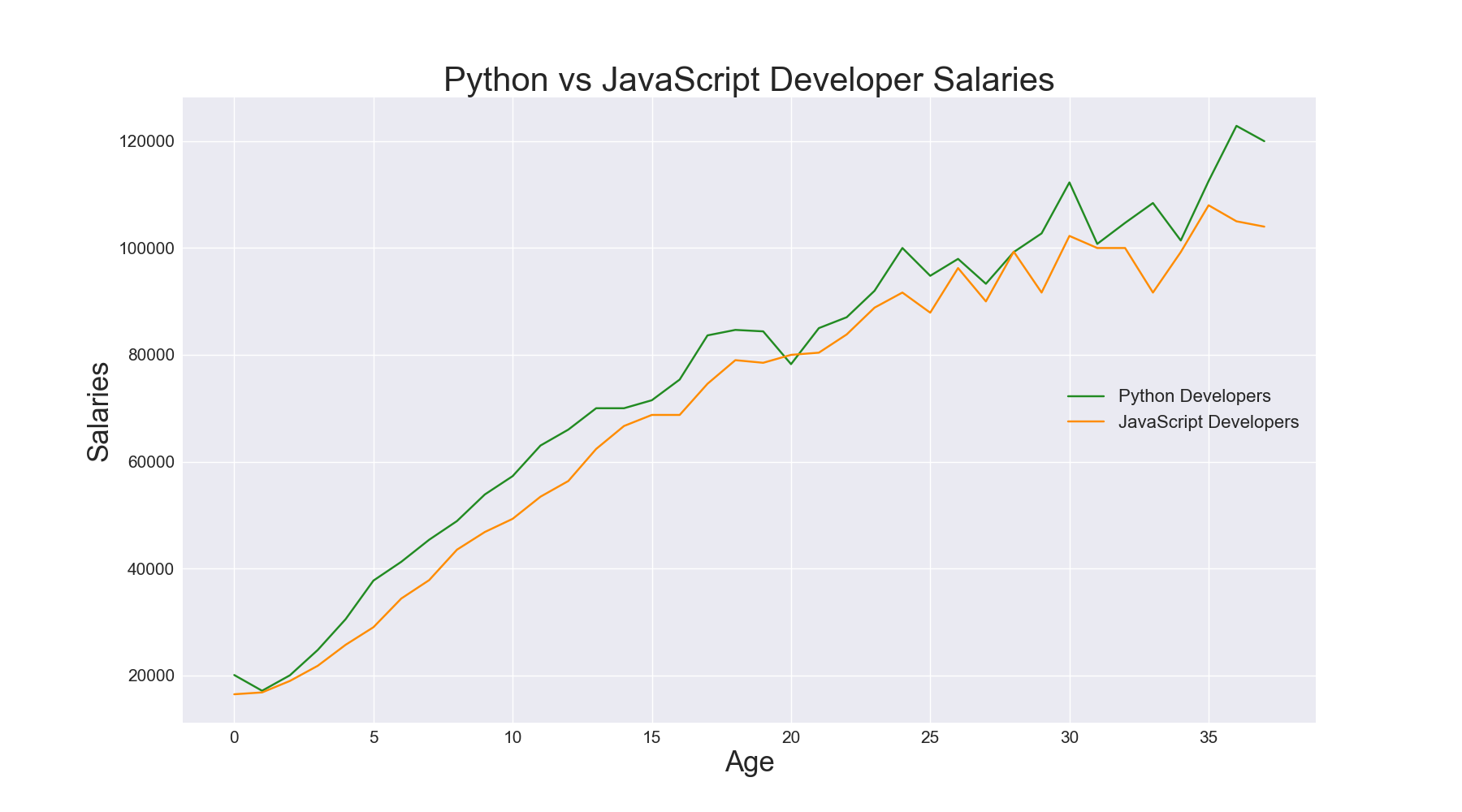
Everything Should Have a Label
Here we are using Matplotlib, but we have added a single color for each line, a title, x and y labels, and a legend for clear concise interpretation.
Every variable has a home, and it sparks joy now, right? — Think how would Marie Kondo code.
Simple, but clear.
Overall, pretty simple right? Well, now you have no excuses for those ugly basic plots. I hope you found this helpful and mayb a little bit fun. There’s so much more on color and design in the documentation, so once you’ve mastered these quick tips, dive in on the documentation below!
In this post I would like to describe in detail our setup and development environment (hardware & software) and how to get it, step by step.
I have been using this setup for more than 5 years with little changes (mainly hardware improvements), in many companies, and helped me in the development of dozens of Data projects. Never missed a single feature while using it. This is the standard setup both Pedro and me use at WhiteBox.
Why this guide? Over time, we found many students and fellow Data Scientists looking for a solid environment with some fundamental features:
Standard Data Science tools like Python, R, and its libraries are easy to install and maintain.
Most libraries just work out of the box with little extra configuration.
Allows to cover the full spectrum of Data related tasks, from Small to Big Data, and from standard Machine Learning models to Deep Learning prototyping.
Do not need to break your bank account to buy expensive hardware and software.
Hardware
Your laptop should have:
At least 16GB of RAM. This is the most important feature as it will limit the amount of data you can easily process in memory (without using tools like Dask or Spark). The more the better. Go with 32GB if you can afford it.
A powerful processor. At least an Intel i5 or i7 with 4 cores. It will save you a lot of time while processing data for obvious reasons.
A NVIDIA GPU of at least 4GB of RAM. Only if you need to prototype or fine-tune simple Deep Learning models. It will be orders of magnitude faster than almost any CPU for that task. Remember that you can’t train serious Deep Learning models from scratch in a laptop.
A good cooling system. You are going to run workloads for at least hours. Make sure your laptop can handle it without melting.
A SSD of at least 256GB should be enough.
Possibility to upgrade its capabilities, like adding a bigger SSD, more RAM, or easily replace battery.
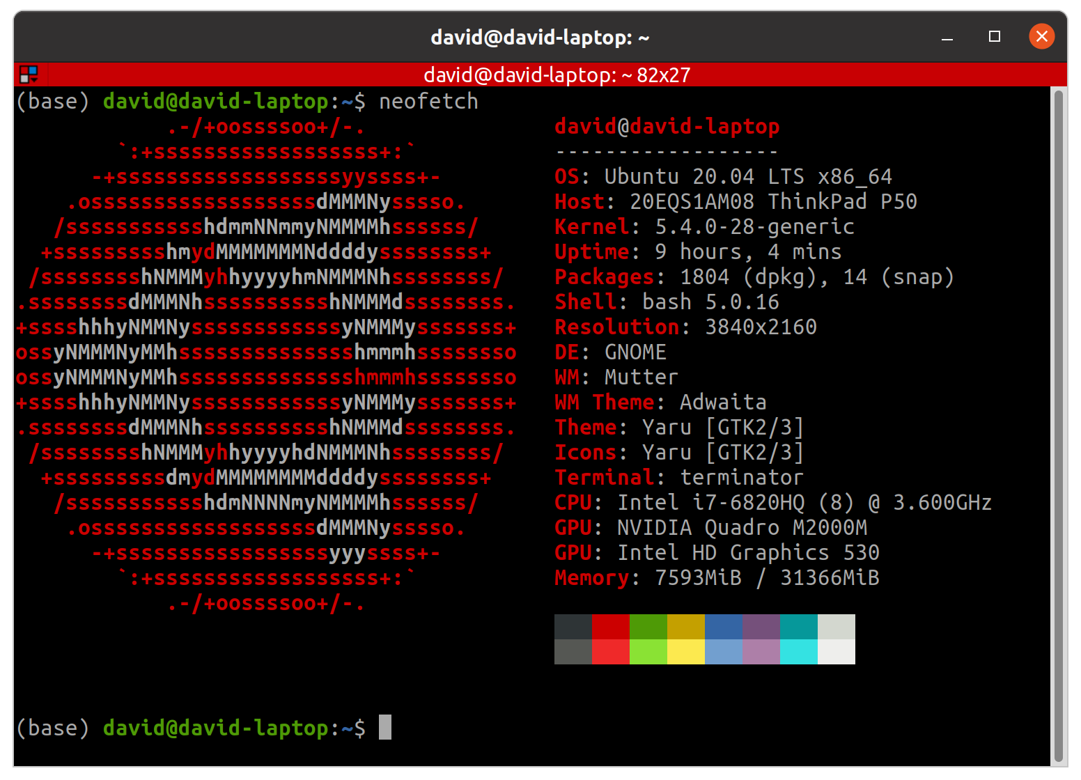
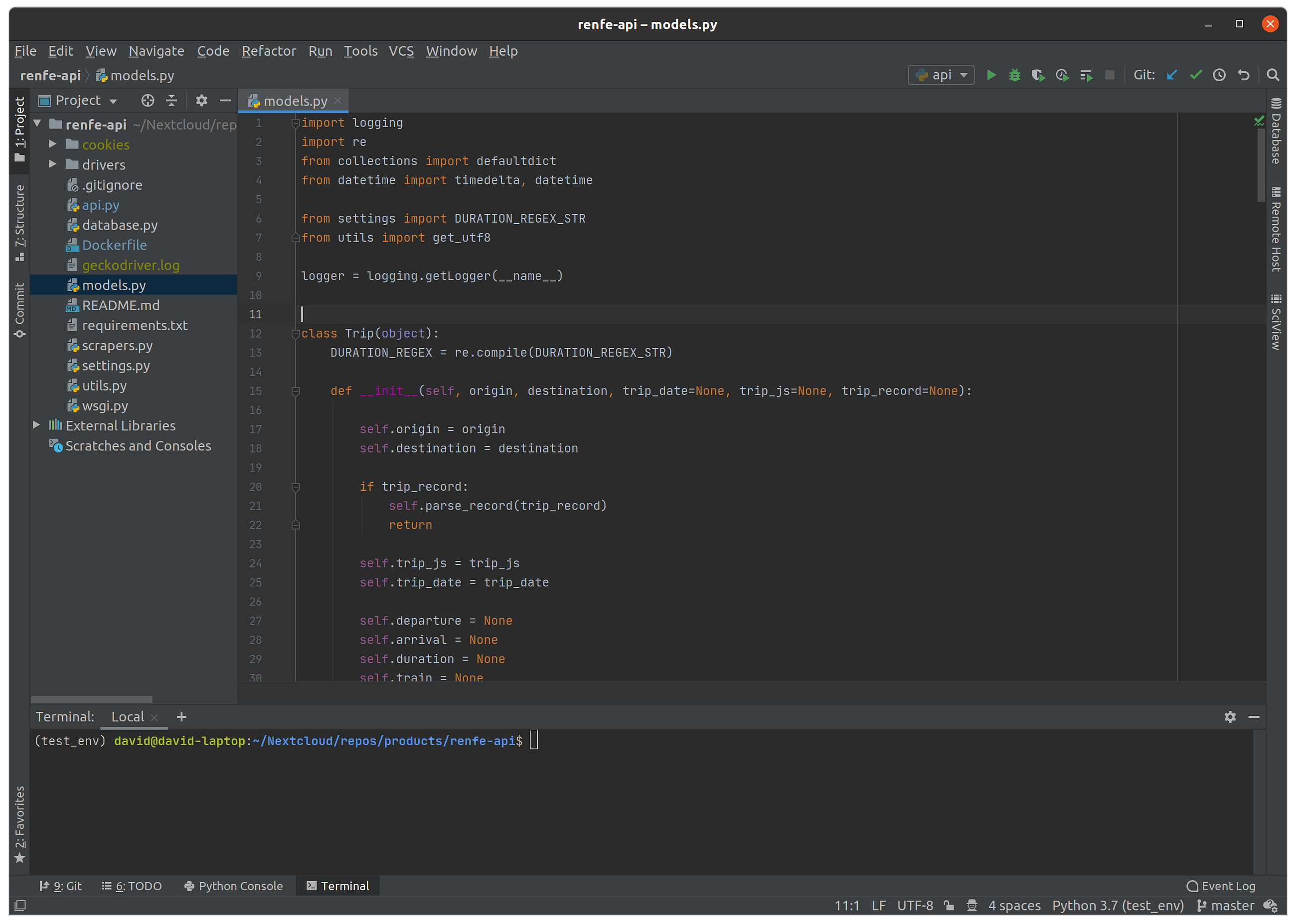
My personal recommendation is getting a second hand Thinkpad workstation laptop. I have an second hand P50 I bought for 500€ which meets all features listed above:
david-laptop specs
Thinkpads are excellent professional laptops we have been using for years and never failed us. Its handicap is the price, but you can find lots of second hand Thinkpads in very good using conditions as many big corporations have leasing agreements and dispose laptops every 2 years. Many of these laptops end in the second hand market. You can start your search in:
Many of these second hand markets can provide warranty and an invoice (in case you are a company). If you are reading this post and belong to a middle to big sized organization, the best option for you is probably reaching a leasing agreement directly with the manufacturer.
Lenovo Thinkpad P52
Avoid Apple MacBooks:
For a variety of reasons, you should avoid an Apple laptops unless you really (and I mean, really) love OSX. They are intended for professionals from the design field and music producers, like photographers, video and photo editors, UX/UI, and even developers who don’t need to run heavy workloads, like Web Developers. My main laptop from 2011 to 2016 was a MacBook, so I know its limitations very well. Main reasons not to buy one are:
You are going to pay much more for the same hardware.
You will suffer a terrible vendor lock-in, which means a huge cost to change to other alternative.
You can’t have a NVIDIA GPU, so forget about Deep Learning prototyping in your laptop.
Can not upgrade its hardware as it is soldered to the motherboard. In case you need more RAM, you have to buy a new laptop.
Avoid Ultrabooks (in general):
Most ultrabooks are designed for light workloads, web browsing, office productivity software and similar. Most of them does not meet the cooling system requirement listed above, and its life will be short. They are also not upgradable.
Operating System
Our go-to operating system for Data Science is the latest LTS (Long Term Support) of Ubuntu. At the time of writing this post, Ubuntu 20.04 LTS is the latest.
Ubuntu 20.04 LTS
Ubuntu offers some advantages over other operating systems and other Linux distros for you as a Data Scientist:
Most successful Data Science tools are open-source and are easy to install and use in Ubuntu, which is also free an open-source. It makes sense as most developers of those tools are probably using Linux. It is specially true when it comes to Deep Learning frameworks with GPU support, like TensorFlow, PyTorch, etc.
As you are going to be working with Data, security must be at the core of your setup. Linux is by default, more secure than Windows or OS X, and as it is used by a minority of people, most malicious software is not designed to run on Linux.
It is the most used Linux distro, both for desktops and servers, with a great and supportive community. When you find something is not working well, it will be easier to get help or find info about how to fix it.
Most servers are Linux based, and you probably want to deploy your code in those servers. The closer you are to the environment you are going to deploy to production, the better. This is one of the main reasons to use Linux as your platform.
It has a great package manager you can use to install almost everything.
Some caveats to install Ubuntu:
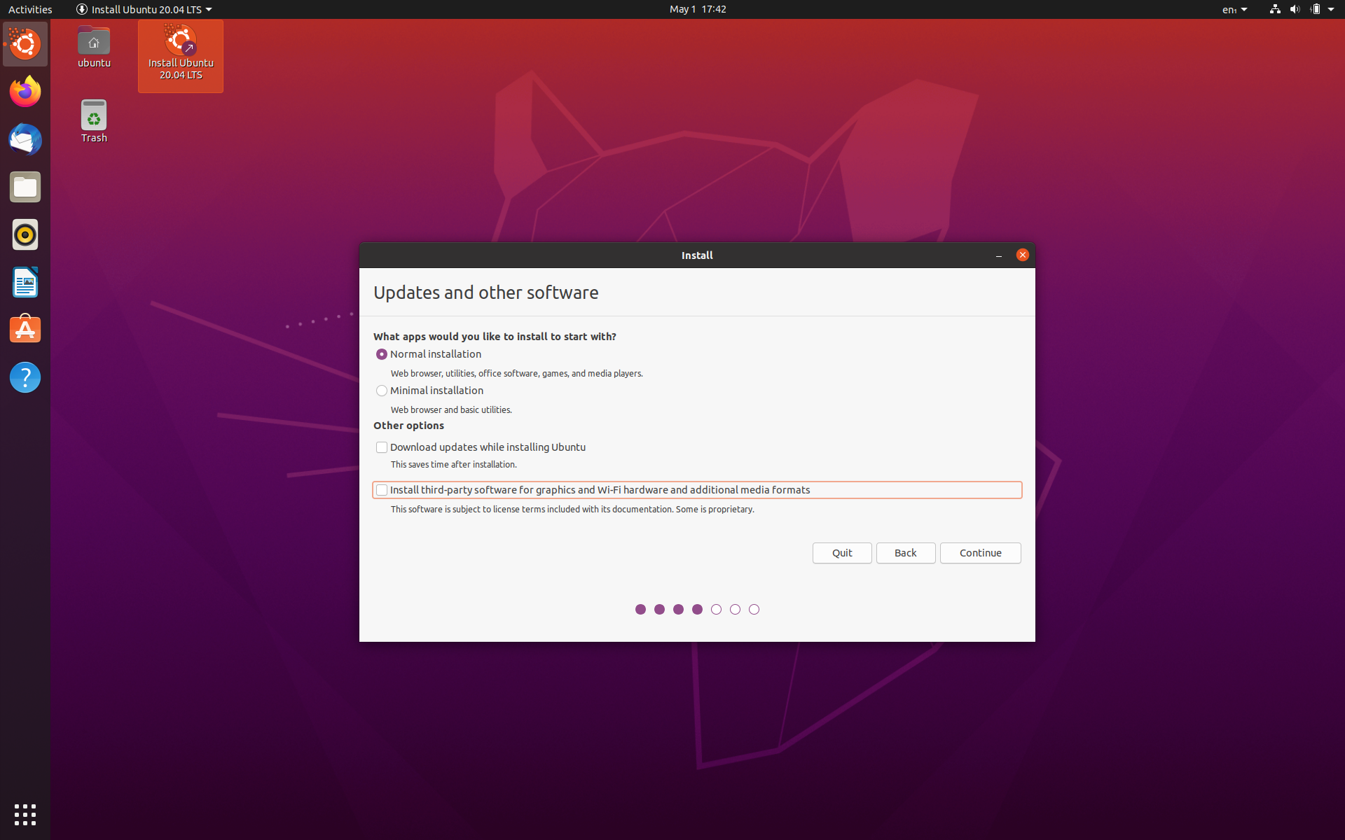
If you are lucky enough to have a dedicated GPU, do not install proprietary drivers for graphics (unchecked box while installation). You can install later as default drivers are buggy and may cause external monitors to not work properly for certain GPU’s (like in my case):
Uncheck third-party software while installation
Create your installation USB properly, if you have access to Linux, can use Startup Disk Creator, for Windows or OSX, balenaEtcher is a solid choice.
NVIDIA Drivers
NVIDIA Linux support has been one of the complaints of the community for years. Remember that famous:
NVIDIA: FUCK YOU!
Linus Torvalds talking about NVIDIA
Luckily, things have changed and now, although still a pain in the ass sometimes, everything is easier.
2. Install latest available drivers (440 at the time of writing this post, use TAB key to check for available options):
sudo apt install nvidia-driver-440
Wait for the installation to finish and reboot your PC.
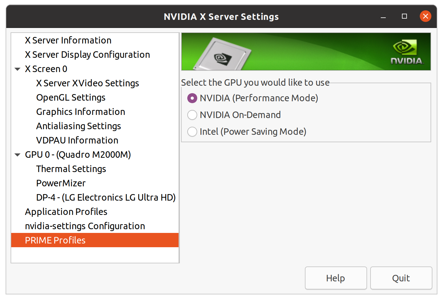
You should be able now to access NVIDIA X Server Settings:
You can use this to switch between Power Saving Mode (useful if you are not going to do any Deep Learning Stuff) and Performance Mode (allows you to use GPU, but drains your battery). Avoid On-Demand mode as it is still not working properly.
NVIDIA X Server Settings
You should also be able to run nvidia-smi application, which displays information about GPU workloads (usage, temperature, memory). You are going to use it a lot while training Deep Learning models on GPU.
nvidia-smi
Terminal
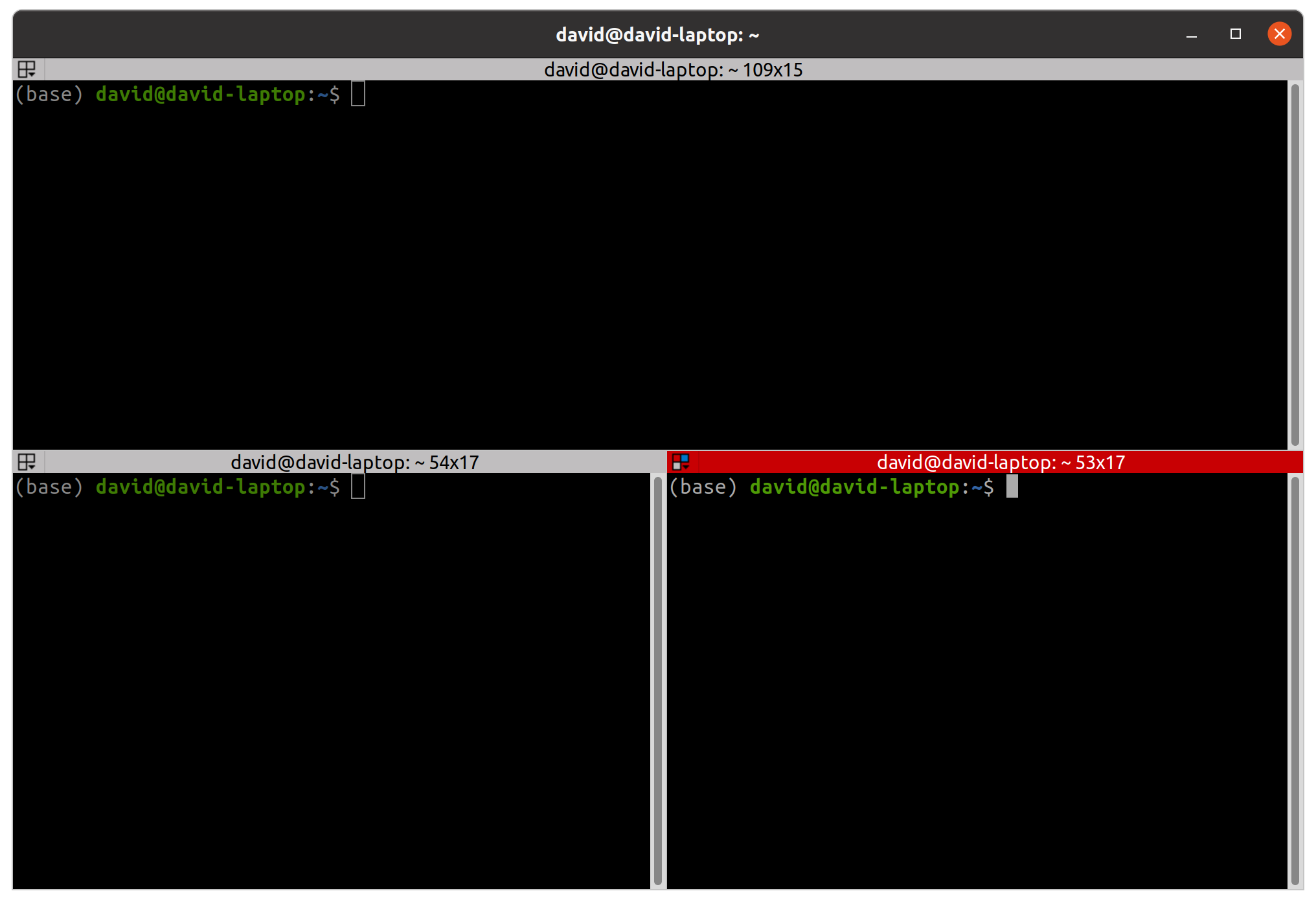
While default GNOME Terminal is OK, I prefer using Terminator, a powerful terminal emulator which allows you to split the terminal window vertically ctr + shift + e and horizontally ctr + shift + o, as well as broadcasting commands to several terminals at the same time. This is useful to setup various servers or a cluster.
Terminator
Install Terminator like this:
sudo apt install terminator
VirtualBox
VirtualBox is a software that allows you to run virtually other machines inside your current operating system session. You can also run different operating systems (Windows inside Linux, or the other way around).
It is useful in case you need a specific software which is not available for Linux, like BI and Dashboarding tools like:
VirtualBox is also useful to test new libraries and software without compromising your system, as you can just create a VM (Virtual Machine), test whatever you need and delete it.
To install VirtualBox, open your terminal and write:
sudo apt install virtualbox
Although its usage is fairly simple, it is hard to master. For an extensive tutorial of VirtualBox, check this.
Python, R and more (with Miniconda)
Python is already included with Ubuntu. But you should never use system Python or install your analytics libraries system-wide. You can break system Python doing that, and fixing it is hard.
I prefer creating isolated virtual environments I can just delete and create again in case something goes wrong. The best tool you can use to do that is conda:
Package, dependency and environment management for any language-Python, R, Ruby, Lua, Scala, Java, JavaScript, C/ C++, FORTRAN, and more.
Although many people uses conda, few people really understand how it works and what it does. It may lead to frustration.
conda is shipped in two flavors:
Anaconda: includes conda package manager and a lot of libraries (500Mb) installed. You are not going to use all those libraries and moreover will be outdated in a few days. I do not recommend going with this flavor.
Miniconda: includes just conda package manager. You still have access to all existing libraries through conda or pip, but those libraries will be downloaded and installed when they are needed. Go with this option, as it will save you time and memory.
Download Miniconda install script from here and run it:
bash Miniconda3-latest-Linux-x86_64.sh
Make sure you initialize conda (so answer yes when install script asks!) and those lines are added to your .bashrc file:
# >>> conda initialize >>>
# !! Contents within this block are managed by 'conda init' !!
__conda_setup="$('/home/david/miniconda3/bin/conda' 'shell.bash' 'hook' 2> /dev/null)"
if [ $? -eq 0 ]; then
    eval "$__conda_setup"
else
    if [ -f "/home/david/miniconda3/etc/profile.d/conda.sh" ]; then
        . "/home/david/miniconda3/etc/profile.d/conda.sh"
    else
        export PATH="/home/david/miniconda3/bin:$PATH"
    fi
fi
unset __conda_setup
# <<< conda initialize <<<
This will add the conda app to your PATH so you can access it anytime. To check conda is properly installed, just type conda in your terminal:
conda help
Remember that in a conda virtual environment you can install whatever Python version you want, as well as R, Java, Julia, Scala, and more…
Remember that you can also install libraries from both conda and pip package managers and don’t have to choose one of them as they are perfectly compatible in the same virtual environment.
One more thing about conda:
conda offers a unique feature for deploying your code. It is a library called conda-pack and it is a must for us. It helped us many times to get our libraries deployed in internet isolated clusters with no access to pip, no python3 and no simple way to install anything you need.
This library allows you to create a .tar.gz file with your environment you can just uncompress wherever you want. Then you can just activate the environment and use it as usual.
This is the ultimate weapon against lazy IT guys who don’t give you the right permissions to work in a given environment and don’t have time to configure it to suit your project needs. Have ssh access to a server? Then you have the environment you want and need.
Jupyter is a must for a Data Scientist, for developments where you need an interactive programming environment.
A trick I learned over the years is to create a local JupyterHub server and configure as a system service so I don’t have to launch the server every time (it is always up and waiting as soon as the laptop starts). I also install a library that detects Python/R kernels in all my environments and automatically make them available in Jupyter.
To do this:
1. First create a conda virtual environment (I usually call it jupyter_env):
8. Enable jupyterhub service, so it starts automatically at boot time:
sudo systemctl enable jupyterhub
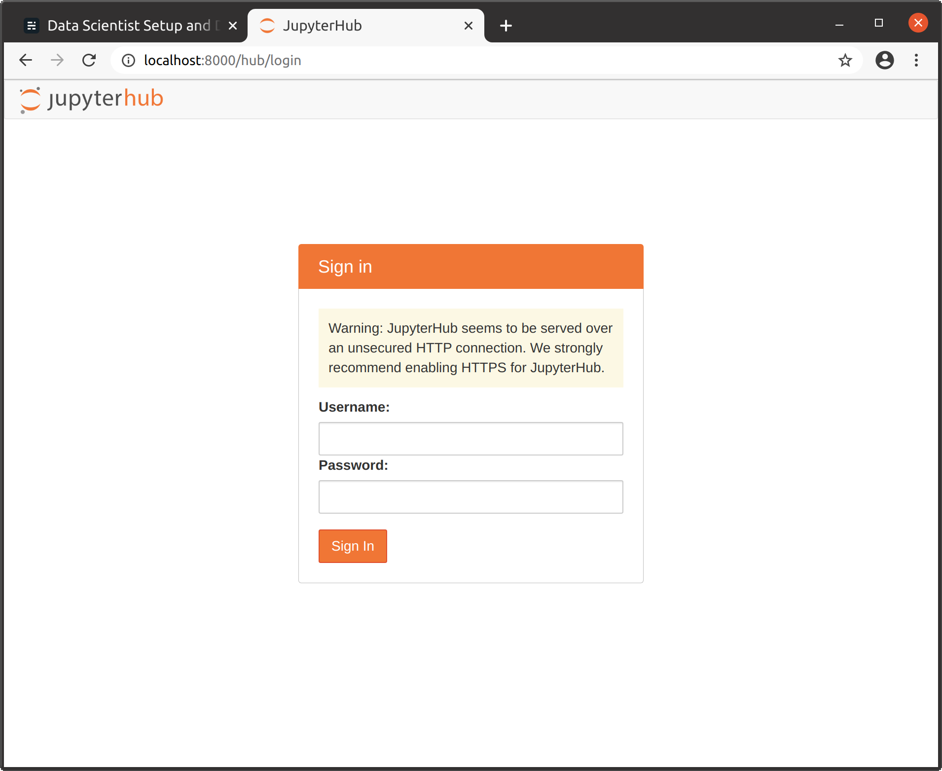
9. Now you can go to localhost:8000 and login with your Linux user and password:
JupyterHub login page
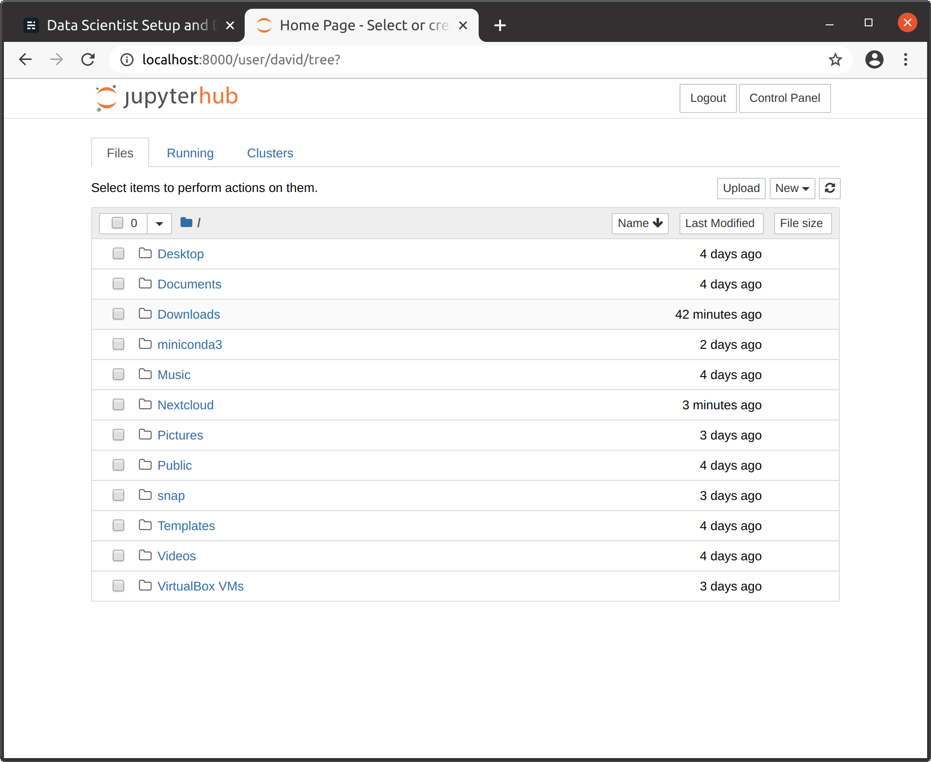
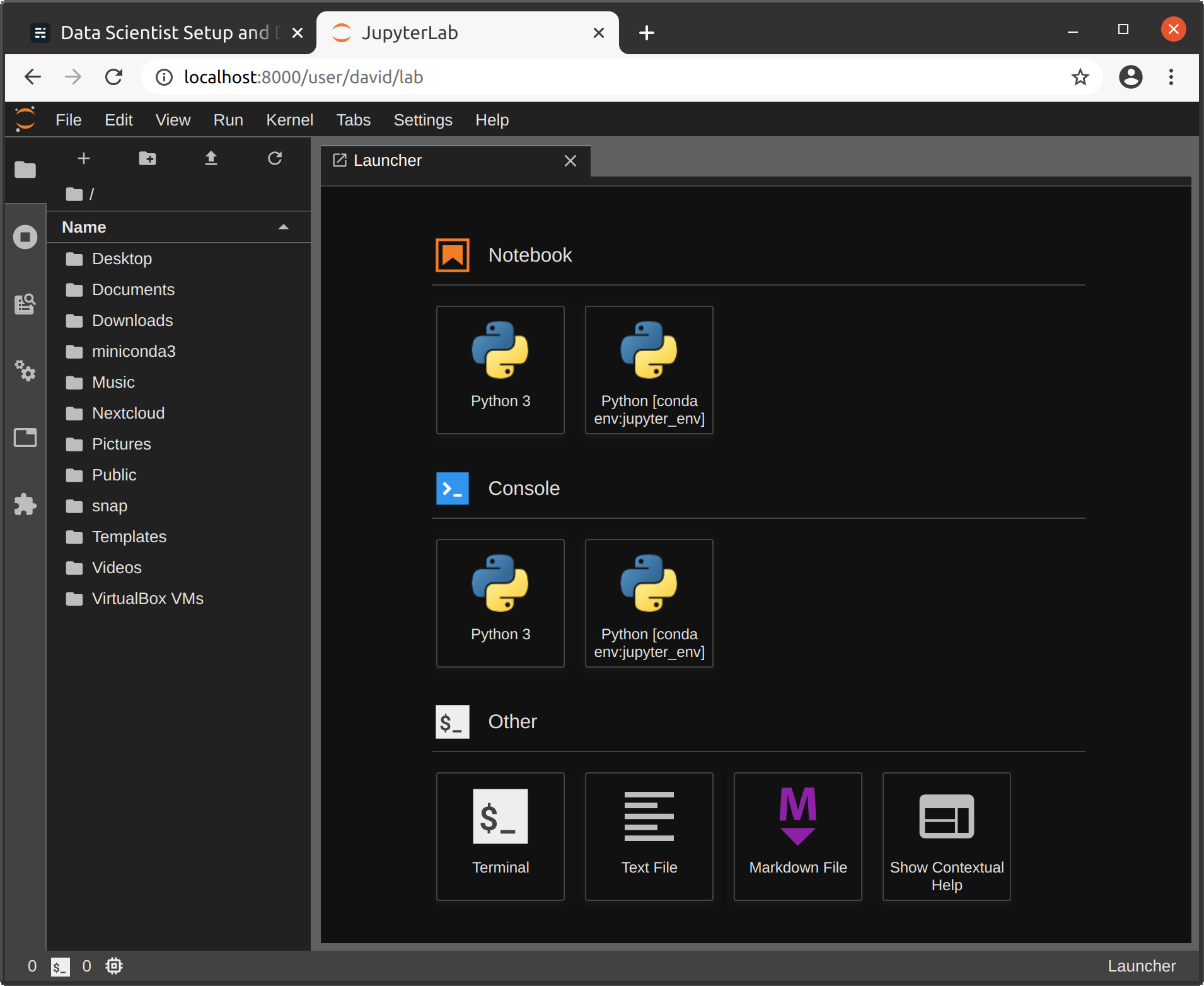
10. After login you have access to a fully fledged Jupyter server at classic mode (/tree) or the more recent JupyterLab (/lab):
Jupyter (Classic)
Jupyter (Lab)
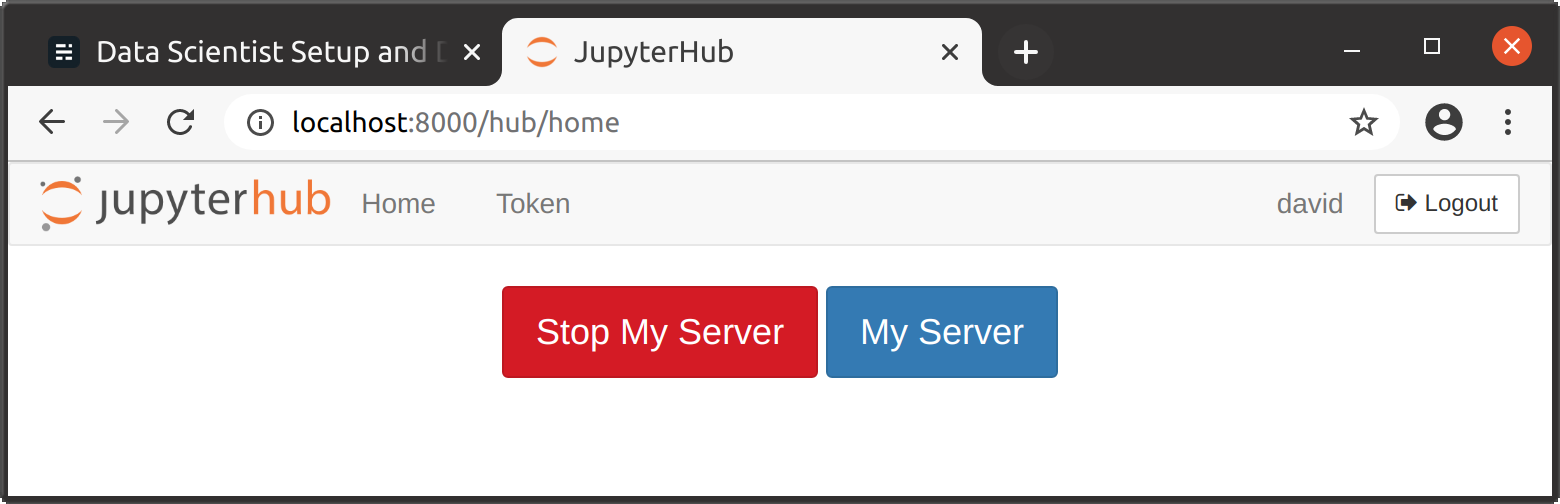
The most interesting feature of this Jupyter setup is that it detects kernels in all conda environments, so you can access those kernels from here with no hassle. Just install the corresponding kernel in the desired environment ( conda install ipykernel, or conda install irkernel) and restart Jupyter server from JupyterHub control panel:
JupyterHub control panel
Remember to previously activate the environment where you want to install the kernel! ( conda activate <env_name>).
As you probably know I am a supporter of FOSS solutions, specially in the Data ecosystem. One of the few proprietary software I am going to recommend here, is the one we use as IDE: PyCharm. If you are serious about your code, you want to use an IDE like PyCharm:
Code completion and environment introspection.
Python environments, including native conda support.
Debugger.
Docker integration.
Git integration.
Scientific mode (pandas DataFrame and NumPy arrays inspection).
PyCharm Professional
Other popular choices does not have the stability and features of Pycharm:
Visual Studio Code: is more a Text Editor than an IDE. I know you can extend it using plugins, but is not as powerful as PyCharm. If you are a Web Dev with projects in multiple languages, Visual Studio Code may be a good choice for you. If you are a Web Developer and Python is your language of choice for back-end, go with Pycharm even if you are not in Data.
Jupyter: if you have doubts about when you should be using Jupyter or PyCharm and call yourself a Data <whatever>, please attend one of the bootcamps we teach asap.
Our advice for installing PyCharm is using Snap, so your installation will be automatically updated and isolated from the rest of the system. For community (free) version:
sudo snap install pycharm-community --classic
Scala
Scala is a language we use for Big Data projects with native Spark, although we are shifting to PySpark.
Our recommendation here is IntelliJ IDEA. It is an IDE for JVM based languages (Java, Kotlin, Groovy, Scala) from PyCharm developers (JetBrains). It best feature is its native support for Scala and its similarities to PyCharm. If you came from Eclipse, can adapt key bindings and shortcuts to replicate Eclipse ones.
Okay, you are not going to really do Big Data in your laptop. In case you are in a Big Data project, your company or client is going to provide you with a proper Hadoop cluster.
But there are situations where you may want to analyze or make a model with data that doesn’t fit easily in your laptop memory. In those cases, a local Spark installation is very helpful. Using my humble laptop, I have crushed datasets sized GB on disk, which on memory translates in much more.
This is our recommendation to get Spark up and running in your laptop:
Dask: simplifying things a lot, Dask is some kind of native Spark for Python. It is closer to pandas and NumPy APIs, but in our experience, it is not as robust as Spark by far. We use it from time to time.
Modin: replicates pandas API with support for multi-core and out-of-core computations. It is specially useful when you are working in a powerful analytics server with lots of cores (32, 64) and want to use pandas. As per-core performance is usually poor, Modin will allow you to speed your computation.
Database Tools
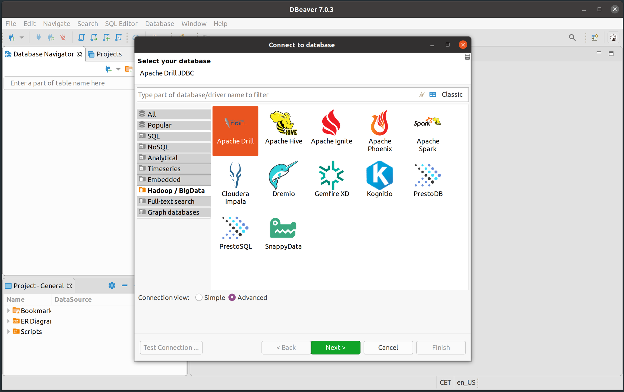
Sometimes you need a tool able to connect with a variety of different DB technologies, make queries and explore data. Our choice is DBeaver:
DBeaver Community
DBeaver is a tool that automatically downloads drivers for lots of different databases. It supports:
Database, schema, table and column name completion.
Advanced networking requirements to connect, like SSH tunnels and more.
You can install DBeaver like this:
sudo snap install dbeaver-ce
Honorable mention:
DataGrip: a database IDE by JetBrains we use sometimes, very similar to DBeaver, with less technologies supported, but very stable: sudo snap install datagrip --classic
Others
Other specific tools and apps that are important for us are:
And this is all. Those are a lot of tools and we probably forgot something. In case you miss some category here or need some advice, leave a comment and we will try to extend the post.
Data is key for any analysis in data science, be it inferential analysis, predictive analysis, or prescriptive analysis. The predictive power of a model depends on the quality of the data that was used in building the model. Data comes in different forms such as text, table, image, voice or video. Most often, data that is used for analysis has to be mined, processed and transformed to render it to a form suitable for further analysis.
The most common type of dataset used in most of the analysis is clean data that is stored in a comma-separated value (csv) table. However because a portable document format (pdf) file is one of the most used file formats, every data scientist should understand how to extract data from a pdf file and transform the data into a format such as “csv” that can then be used for analysis or model building.
Copying data from a pdf file line by line is too tedious and can often lead to corruption due to human errors during the process. It is therefore extremely important to understand how to import data from a pdf in an efficient and error-free manner.
In this article, we shall focus on extracting a data table from a pdf file. A similar analysis can be made for extracting other types of data such as text or an image from a pdf file. This article focuses on extracting numerical data from a pdf file. For extraction of images from a pdf file, python has a package called minecart that can be used for extracting images, text, and shapes from pdfs.
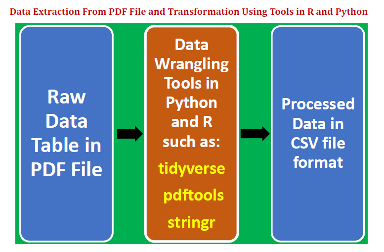
We illustrate how a data table can be extracted from a pdf file and then transformed into a format appropriate for further analysis and model building. We shall present two examples, one using Python, and the other using R. This article will consider the following:
Extract a data table from a pdf file.
Clean, transform and structure the data using data wrangling and string processing techniques.
Store clean and tidy data table as a csv file.
Introduce data wrangling and string processing packages in R such as “tidyverse”, “pdftools”, and “stringr”.
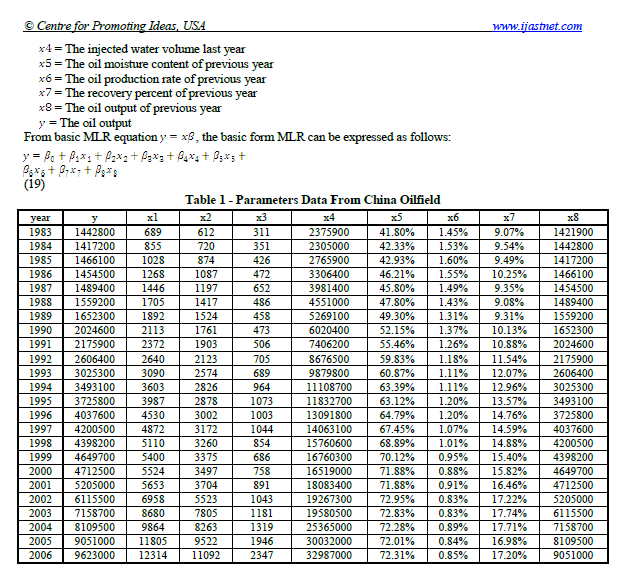
Example 1: Extract a Table from PDF File Using Python
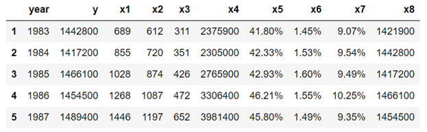
Let us suppose we would like to extract the table below from a pdf file.
— — — — — — — — — — — — — — — — — — — — — — — — —
— — — — — — — — — — — — — — — — — — — — — — — — —
a) Copy and past table to Excel and save the file as table_1_raw.csv
Data is stored in one-dimensional format and has to be reshaped, cleaned, and transformed.
We note that column values for columns x5, x6, and x7 have data types of string, so we need to convert these to numeric data as follows:
df4['x5']=[float(x) for x in df4['x5'].values]df4['x6']=[float(x) for x in df4['x6'].values]df4['x7']=[float(x) for x in df4['x7'].values]
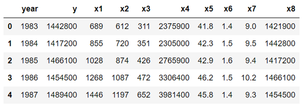
f) View final form of the transformed data
df4.head(n=5)
g) Export final data to a csv file
df4.to_csv('table_1_final.csv',index=False)
Example 2: Extract a Table From PDF File Using R
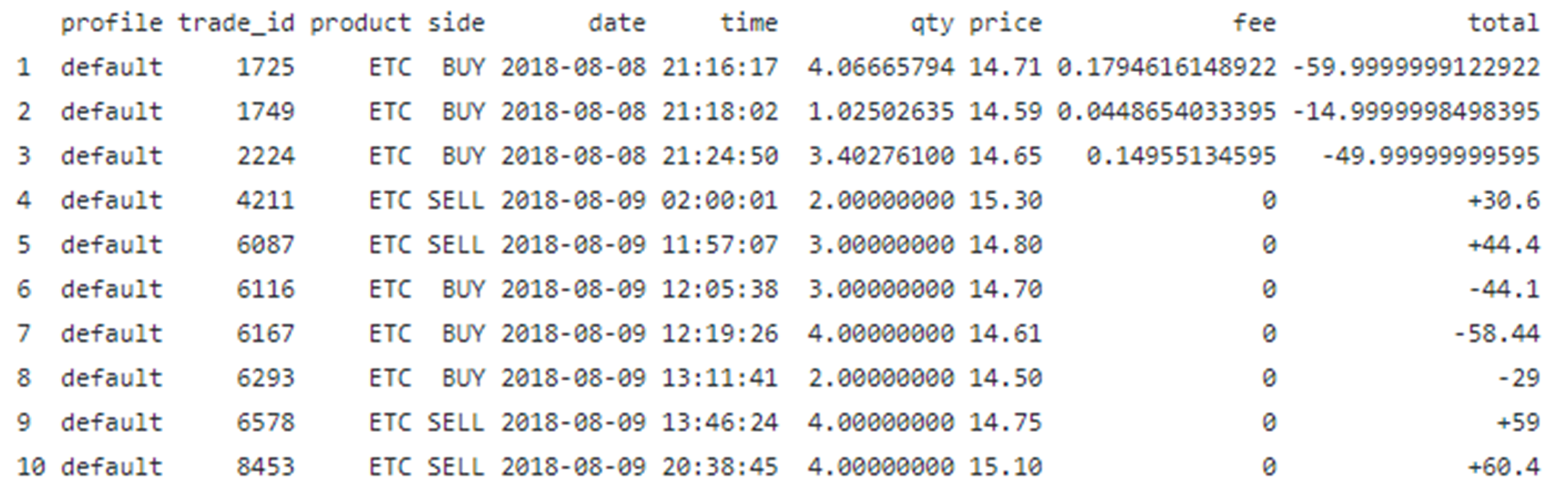
This example illustrates how to extract a table from a pdf file using data wrangling techniques in R. Let us suppose we have the following table from a pdf file name trade_report.pdf:
— — — — — — — — — — — — — — — — — — — — — — — — —
— — — — — — — — — — — — — — — — — — — — — — — —
We would like to extract the table, wrangle the data, and convert it to a data frame table ready for further analysis. The final data table can then be easily exported and stored in a “csv” file. In particular, we would like to accomplish the following:
i) On the column Product, we would like to get rid of USD from the product ETC-USD.
ii) Split the Date column into two separate columns, namely, date and time.
In summary, we’ve shown how a data table can be extracted from a pdf file. Since a pdf file is a very common file type, every data scientist should be familiar with techniques for extracting and transforming data stored in a pdf file.
An iterator is an object with a __next__ method. It has a state. The state is used to remember the execution during iteration. Therefore an iterator knows about its current state and this makes it memory efficient. This is the reason why an iterator is used in memory efficient and fast applications.
We can open an infinite stream of data (such as reading a file) and get the next item (such as the next line from the file). We can then perform an action on the item and proceed to the next item. This could mean that we can have an iterator that returns an infinite number of elements as we only need to be aware of the current item.
It has a __next__ method that returns the next value in the iteration and then updates the state to point to the next item. The iterator will always get us the next item from the stream when we execute next(iterator)
When there is no next item to be returned, the iterator raises a StopIteration exception.
As a result, a lean application can be implemented by using iterators
Note, collections such as a list, string, file lines, dictionary, tuples, etc. are all iterators.
Quick Note: What Is An Iterable?
An iterable is an object that can return an iterator. It has an __iter__ method that returns an iterator.
An iterable is an object which we can loop over and can call iter() on. It has a __getitem__ method that can take sequential indexes starting from zero (and raises an IndexError when the indexes are no longer valid).
Itertools is a Python module that is part of the Python 3 standard libraries. It lets us perform memory and computation efficient tasks on iterators. It is inspired by constructs from APL, Haskell, and SML.
Essentially, the module contains a number of fast and memory-efficient methods that can help us build applications succinctly and efficiently in pure Python.
Python’s Itertool is a module that provides various functions that work on iterators to produce iterators. It allows us to perform iterator algebra.
The most important point to take is that the itertools functions can return an iterator.
This brings us to the core of the article. Let’s understand how infinite iterators work.
1. Infinite Iterators
What if we want to construct an iterator that returns an infinite evenly spaced values? Or, what if we have to generate a cycle of elements from an iterator? Or, maybe we want to repeat the elements of an iterator?
The itertools library offers a set of functions which we can use to perform all of the required functionality.
The three functions listed in this section construct and return iterators which can be a stream of infinite items.
Count
As an instance, we can generate an infinite sequence of evenly spaced values:
start = 10
stop = 1
my_counter = it.count(start, stop)
for i in my_counter:
    # this loop will run for ever
    print(i)
This will print never-ending items e.g.
10 11 12 13 14 15
Cycle
We can use the cycle method to generate an infinite cycle of elements from the input.
The input of the method needs to be an iterable such as a list or a string or a dictionary, etc.
my_cycle = it.cycle('Python')
for i in my_cycle:
    print(i)
This will print never-ending items:
P y t h o n P y t h o n P
Repeat
To repeat an item (such as a string or a collection), we can use the repeat() function:
to_repeat = 'FM'
how_many_times = 4
my_repeater = it.repeat(to_repeat, how_many_times)
for i in my_repeater:
    print(i)#Prints
FM
FM
FM
FM
This will repeat the string ‘FM’ 4 times. If we do not provide the second parameter then it will repeat the string infinite times.
In this section, I will illustrate the powerful features of terminating iterations. These functions can be used for a number of reasons, such as:
We might have a number of iterables and we want to perform an action on the elements of all of the iterables one by one in a single sequence.
Or when we have a number of functions which we want to perform on every single element of an iterable
Or sometimes we want to drop elements from the iterable as long as the predicate is true and then perform an action on the other elements.
Chain
This method lets us create an iterator that returns elements from all of the input iterables in a sequence until there are no elements left. Hence, it can treat consecutive sequences as a single sequence.
chain = it.chain([1,2,3], ['a','b','c'], ['End'])
for i in chain:
    print(i)
This will print:
1 2 3 a b c End
Drop While
We can pass an iterable along with a condition and this method will start evaluating the condition on each of the elements until the condition returns False for an element. As soon as the condition evaluates to False for an element, this function will then return the rest of the elements of the iterable.
As an example, assume that we have a list of jobs and we want to iterate over the elements and only return the elements as soon as a condition is not met. Once the condition evaluates to False, our expectation is to return the rest of the elements of the iterator.
jobs = ['job1', 'job2', 'job3', 'job10', 'job4', 'job5']
dropwhile = it.dropwhile(lambda x : len(x)==4, jobs)
for i in dropwhile:
    print(i)
This method will return:
job10 job4 job5
The method returned the three items above because the length of the element job10 is not equal to 4 characters and therefore job10 and the rest of the elements are returned.
The input condition and the iterable can be complex objects too.
Take While
This method is the opposite of the dropwhile() method. Essentially, it returns all of the elements of an iterable until the first condition returns False and then it does not return any other element.
As an example, assume that we have a list of jobs and we want to stop returning the jobs as soon as a condition is not met.
jobs = ['job1', 'job2', 'job3', 'job10', 'job4', 'job5']
takewhile = it.takewhile(lambda x : len(x)==4, jobs)
for i in takewhile:
    print(i)
This method will return:
job1 job2 job3
This is because the length of ‘job10’ is not equal to 4 characters.
GroupBy
This function constructs an iterator after grouping the consecutive elements of an iterable. The function returns an iterator of key, value pairs where the key is the group key and the value is the collection of the consecutive elements that have been grouped by the key.
Consider this snippet of code:
iterable = 'FFFAARRHHHAADDMMAAALLIIKKK'
my_groupby = it.groupby(iterable)
for key, group in my_groupby:
    print('Key:', key)
    print('Group:', list(group))
Note, the group property is an iterable and therefore I materialised it to a list.
As a result, this will print:
Key: F Group: [‘F’, ‘F’, ‘F’] Key: A Group: [‘A’, ‘A’] Key: R Group: [‘R’, ‘R’] Key: H Group: [‘H’, ‘H’, ‘H’] Key: A Group: [‘A’, ‘A’] Key: D Group: [‘D’, ‘D’] Key: M Group: [‘M’, ‘M’] Key: A Group: [‘A’, ‘A’, ‘A’] Key: L Group: [‘L’, ‘L’] Key: I Group: [‘I’, ‘I’] Key: K Group: [‘K’, ‘K’, ‘K’]
We can also pass in a key function as the second argument if we want to group by a complex logic.
Tee
This method can split an iterable and generate new iterables from the input. The output is also an iterator that returns the iterable for the given number of items. To understand it better, review the snippet below:
iterable = 'FM'
tee = it.tee(iterable, 5)
for i in tee:
    print(list(i))
This method returned the entire iterable FM, 5 times:
This article explained the uses of the Itertools library. In particular, it explained:
Infinite Iterators
Terminating Iterators
Combinatoric Iterators
The itertools methods can be used in combination to serve a powerful set of functionality in our applications. We can use the Itertools library to implement precise, memory efficient and stable applications in a shorter time.
I recommend potentially evaluating our applications to assess whether we can use the Itertools library.
For more detailed information, please visit the Python official documentation here
Let us imagine you are trying to convince a client to invest in your company. You exhibit all the employee’s records and their achievements in the form of an excel sheet rather than a bar chart or a pie chart. Imagine yourself in the client’s place. How would you react then? (Wouldn’t too much data be so overwhelming?). This is where data visualization comes into the picture.
Data visualization is the practice of translating raw data into visual plots and graphs to make it easier for the human brain to interpret. The primary objective is to make the research and data analysis quicker and also to communicate the trends, patterns effectively.
The human brain is programmed to understand visually appealing data better than lengthy plain texts.
In this article, Let us take a dataset, clean the data as per requirement, and try visualizing the data. The dataset is taken from Kaggle. You can find it here.
Firstly, to load the data from external sources and clean it, we will be using the Pandas library. You can study more about Pandas in my previous article here.
We need to import the Pandas library in-order to use it. We can import it by using it.
import pandas as pd
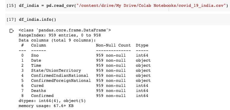
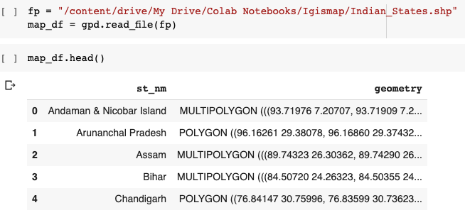
Let us load the CSV file taken from Kaggle and try to know more about it.
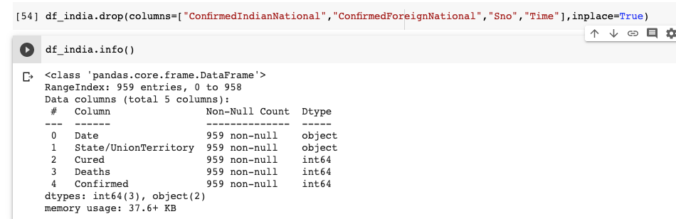
We can understand that the dataset has 9 columns in total. The Date and Time column indicate the last updated date and time. We are not going to use the ConfirmedIndianNational and ConfirmedForeignNational columns. Hence let us drop these 2 columns. The Time column is also immaterial. Let us drop it too. Since the Data Frame already has an index, the Serial No(Sno) column is also not required.
Right away, we can see that the data frame has only 5 columns. It is a good practice to drop redundant data because retaining it will take up unneeded space and potentially bog down runtime.
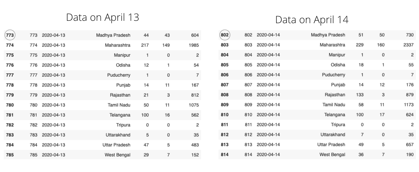
Here the Kaggle dataset is updated daily. New data is appended instead of overwriting the existing data. For instance, on April 13th dataset has 925 rows with each row representing the cumulative data of one particular state. But on April 14th, the dataset had 958 rows, which means 34 new rows(Since there are a total of 34 different states in the dataset) were appended on April 14th.
In the above picture, you can notice the same State names, but try to observe the changes in other columns. Data about new cases are appended to the dataset every day. This form of data can be useful to know the spread trends. Like-
The increment in the number of cases across time.
Performing time series analysis
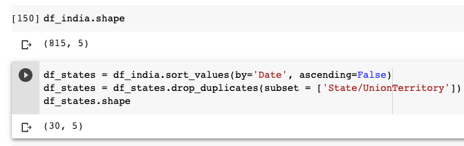
But we are interested in analyzing only the latest data leaving aside the previous data. Hence let us drop those rows which are not required.
Firstly, let us sort the data by date in descending order. And get rid of the duplicate values by grouping data using state name.
You can see that the df_states data frame has only 30 rows, which means there is a unique row showing the latest stats for each state. When we sort the data frame using the date column, we will have data frame sorted according to dates in descending order(observe that ascending=False in code) and remove_duplicates stores the first occurrence of value and removes all its duplicate occurrences.
Let us now talk about data visualization. We will use Plotly to visualize the above data frame.
Histograms, Barplots, Scatter plots explain patterns and trends efficiently, but since we are dealing with geographical data, I prefer choropleth maps.
What are Choropleth maps?
According to Plotly, Choropleth maps depict divided geographical regions that are colored or shaded with respect to a data variable. These maps offer a quick and easy way to show value over a geographical area, unveiling trends and patterns too.
Source — Youtube
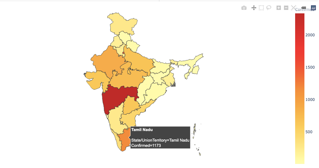
In the above image, areas are colored based on their population density. Darker the color implies higher the population in that particular area. Now with respect to our dataset, we are also going to create a choropleth map based on Confirmed cases. More the number of confirmed cases, darker the color of that particular region.
To render an Indian map, we need a shapefile with the state coordinates. We can download the shapefile for India here.
According to Wikipedia, The shapefile format is a geospatial vector data format for geographic information system (GIS).
Before working with shapefiles, we need to install GeoPandas, which is a python package that makes work with geospatial data easy.
pip install geopandas
import geopandas as gpd
You can see that the data frame has a State name and its coordinates in vector form. Now we will convert this shapefile into the required JSON format.
import json#Read data to json.merged_json = json.loads(map_df.to_json())
Next, we are going to create Choropleth Maps using Plotly Express.’ px.choropleth function. Making choropleth maps requires geometric information.
This can either be a supplied in the GeoJSON format(which we created above) where each feature has a unique identifying value (like st_nm in our case)
2. Existing geometries within Plotly that include the US states and world countries
The GeoJSON data, i.e. (the merged_json we create above) is passed to the geojson argument and the metric of measurement is passed into the color argument of px.choropleth.
Every choropleth map has a locations argument that takes the State/Country as a parameter. Since we are creating a choropleth map for different states in India, we pass the State column to the argument.
The first parameter is the data frame itself, and the color is going to vary based on the Confirmed value. We set the visible argument in fig.updtae_geos() to False to hide the base map and frame. We also set fitbounds = "locations" to automatically zoom the world map to show our areas of interest.
We can hover across states to know more about them.
Data Visualization is an art that is highly underestimated. Hopefully, you have taken some concepts that will help when visualizing data in real-time. Do feel free to share your feedback and responses. Raise your hands if you’ve learned something new today.