Data Science and Data Proicessing

OPINION

Bye-bye Python. Hello Julia!

As Python’s lifetime grinds to a halt, a hot new competitor is emerging

Woman with hat covering her face in front of sunset
If Julia is still a mystery to you, don’t worry. Photo by Julia Caesar on Unsplash

The Zen of Python versus the Greed of Julia

Beautiful is better than ugly.
Explicit is better than implicit.
Simple is better than complex.
Complex is better than complicated.
Flat is better than nested.
Sparse is better than dense.
Readability counts.
Special cases aren't special enough to break the rules.
Although practicality beats purity.
[...]
ABC paved the way for Python, which is paving the way for Julia. Photo by David Ballew on Unsplash
We are greedy: we want more.We want a language that's open source, with a liberal license. We want the speed of C with the dynamism of Ruby. We want a language that's homoiconic, with true macros like Lisp, but with obvious, familiar mathematical notation like Matlab. We want something as usable for general programming as Python, as easy for statistics as R, as natural for string processing as Perl, as powerful for linear algebra as Matlab, as good at gluing programs together as the shell. Something that is dirt simple to learn, yet keeps the most serious hackers happy. We want it interactive and we want it compiled.

What Julia developers are loving

Versatility

Speed

Community

Code conversion

Image for post
Libraries are still a strong point of Python. Photo by Susan Yin on Unsplash

Libraries

Dynamic and static types

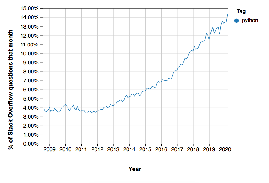
The data: Invest in things while they’re small
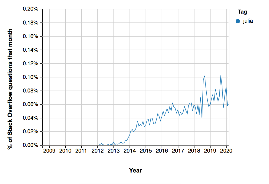
Image for post
Image for post
Number of questions tagged Julia (left) and Python (right) on StackOverflow.
Lots of ones and zeroes on screen, forming a red heart
It’s time to show Julia some love. Photo by Alexander Sinn on Unsplash

Bottom line: Do Julia and let it be your edge

Even though we recognize that we are inexcusably greedy, we still want to have it all. About two and a half years ago, we set out to create the language of our greed. It's not complete, but it's time for a 1.0 release — the language we've created is called Julia. It already delivers on 90% of our ungracious demands, and now it needs the ungracious demands of others to shape it further. So, if you are also a greedy, unreasonable, demanding programmer, we want you to give it a try.

Python Lambda Expressions in Data Science

Upgrade your python coding standards to upgrade your research

Sep 2 · 3 min read
Photo by Max Baskakov on Unsplash

Coding efficiently is one of the key premises to the use case of Python and Lambda expressions are no different. Python lambda’s are anonymous functions which involve small and concise syntax, whereas at times, regular functions can be too descriptive and quite long.

Python is one of a few languages which had lambda functions added to their syntax whereas other languages, like Haskell, uses lambda expressions as a core concept.

Whatever your use-case of a Lambda function, it’s really good to know what they’re about and how to use them.

Why Use Lambda Functions?

The true power of a lambda function can be shown when used inside another function but let’s start on the easy step.

Say you have a function definition that takes one argument, and that argument will be added to an unknown number:

def identity(x):
... return x + 10

However this can be compressed into a simple one-liner as follows:

identity = lambda a : a + 10

This function can then be used as follows:

identity(10) 

which will give the answer 20.

Now with this simple concept, we can also extend this to have more than one input as follows:

myfunc = lambda a, b, c : a + b + c

So the following:

myfunc(2,3,4)

Will give the function 9. It’s really that simple!

Now a really cool use case of Lambda expressions occurs when you use lambda functions within functions. Take the following example:

def myfunc(n):
return lambda a : a * n

Here, the function myfunc returns a lambda function which multiplies the input a by a pre-defined integer, n. This allows the user to create functions on the fly:

mydoubler = myfunc(2)
mytripler = myfunc(3)

As can be seen, the function mydoubler is a function that simply defines an input by the number 2, whereas mytripler multiplies an input by 3. Test it out!

print(mydoubler(11))
print(mytripler(11))

This brings about the answers 22 and 33.

Photo by Ian Stauffer on Unsplash

Are Lambdas Pythonic or Not?

According to the style-guide of Python (PEP 8), it describes the following which actually recommends users TO NOT use Lambda expressions:

Always use a def statement instead of an assignment statement that binds a lambda expression directly to an identifier.

Yes:

def f(x): 
return 2*x

No:

f = lambda x: 2*x

The logic around this is probably more to do with readability than any personal vendetta against lambda expressions. Agreeably, they can make it a bit more difficult to understand the use case but as a coder who prefers efficiency and simplicity in code, I do feel that there’s a place for them.

However, readable code has to be the most important feature of any code — debatably more important than efficiently run code.

Example Math Formulas

Mean:

mu = lambda x: sum(x) / len(x)

Variance:

variance = lambda x: sum((x - mu(x))**2) / (len(x) - 1)

Thanks for reading! If you have any messages, please let me know!

Keep up to date with my latest articles here!

Image for post

The New Jupyter Book

Jupyter Book extends the notebook idea

Aug 25 · 11 min read

2020–08–07 | On the Jupyter blog, Chris Holdgraf announces a rewrite of the Jupyter Book project.

Jupyter Book is an open source project for building beautiful, publication-quality books, websites, and documents from source material that contains computational content. With this post, we’re happy to announce that Jupyter Book has been re-written from the ground up, making it easier to install, faster to use, and able to create more complex publishing content in your books. It is now supported by the Executable Book Project, an open community that builds open source tools for interactive and executable documents in the Jupyter ecosystem and beyond.”

Image for post
Source: https://jupyterbook.org/

What does the new Jupyter Book do?

The new version of Jupyter Book will feel very similar. However, it has a lot of new features due to the new Jupyter Book stack underneath (more on that later).

The new Jupyter Book has the following main features (with links to the relevant documentation for each):

Write publication-quality content in markdown
You can write in either Jupyter markdown, or an extended flavor of markdown with publishing features. This includes support for rich syntax such as citations and cross-references, math and equations, and figures.

Write content in Jupyter Notebooks
This allows you to include your code and outputs in your book. You can also write notebooks entirely in markdown to execute when you build your book.

Execute and cache your book’s content
For .ipynb and markdown notebooks, execute code and insert the latest outputs into your book. In addition, cache and re-use outputs to be used later.

Insert notebook outputs into your content
Generate outputs as you build your documentation, and insert them in-line with your content across pages.

Add interactivity to your book
You can toggle cell visibility, include interactive outputs from Jupyter, and connect with online services like Binder.

Generate a variety of outputs
This includes single- and multi-page websites, as well as PDF outputs.

Build books with a simple command-line interface
You can quickly generate your books with one command, like so: jupyter-book build mybook/

These are just a few of the major changes that we’ve made. For a more complete idea of what you can do, check out the Jupyter Book documentation

An enhanced flavor of markdown

The biggest enhancement to Jupyter Book is support for the MyST Markdown language. MyST stands for “Markedly Structured Text”, and is a flavor of markdown that implements all of the features of the Sphinx documentation engine, allowing you to write scientific publications in markdown. It draws inspiration from RMarkdown and the reStructuredText ecosystem of tools. Anything you can do in Sphinx, you can do with MyST as well.

MyST Markdown is a superset of Jupyter Markdown (AKA, CommonMark), meaning that any default markdown in a Jupyter Notebook is valid in Jupyter Book. If you’d like extra features in markdown such as citations, figures, references, etc, then you may include extra MyST Markdown syntax in your content.

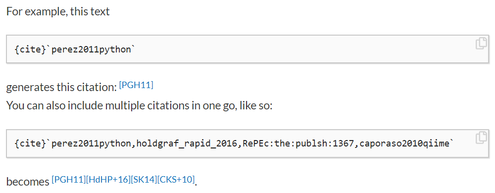
For example, here’s how you can include a citation in the new Jupyter Book:

Image for post
A sample citation. Here we see how you can include citation syntax in-line with your markdown, and then insert a bibliography later on in your page. (source: https://executablebooks.org/)

A smarter build system

While the old version of Jupyter Book used a combination of Python and Jekyll to build your book’s HTML, the new Jupyter Book uses Python all the way through. This means that building the HTML for your book is as simple as:

jupyter-book build mybookname/

In addition, the new build system leverages Jupyter Cache to execute notebook content only if the code is updated, and to insert the outputs from the cache at build time. This saves you time by avoiding the need to re-execute code that hasn’t been changed.

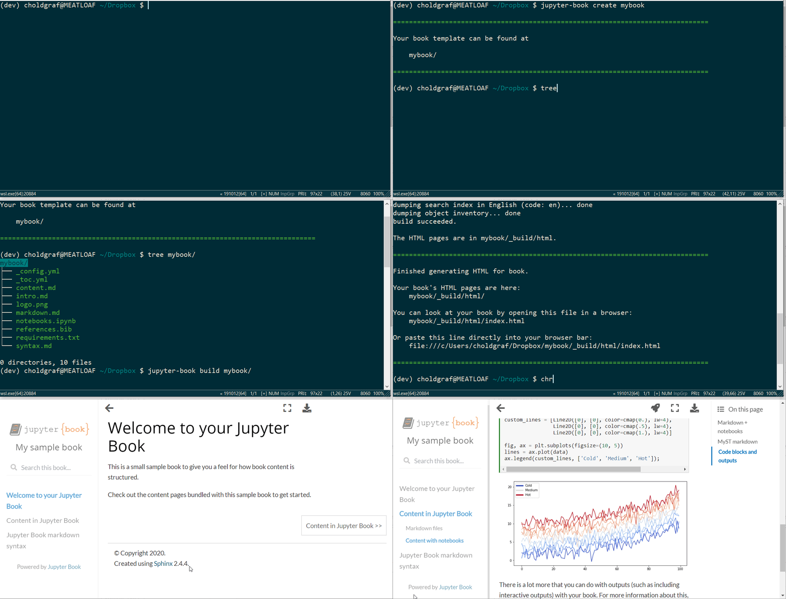
Image for post
An example build process. Here the jupyter-book command-line interface is used to convert a collection of content into an HTML book. (source: https://blog.jupyter.org/)

More book output types

By leveraging Sphinx, Jupyter Book will be able to support more complex outputs than just an HTML website. For example, we are currently prototyping PDF Outputs, both via HTML as well as via LaTeX. This gives Jupyter Book more flexibility to generate the right book for your use case.

You can also run Jupyter Book on individual pages. This means that you can write single-page content (like a scientific article) entirely in Markdown.

A new stack

The biggest change under-the-hood is that Jupyter Book now uses the Sphinx documentation engine instead of Jekyll for building books. By leveraging the Sphinx ecosystem, Jupyter Book can more effectively build on top of community tools, and can contribute components back to the broader community.

Instead of being a single repository, the old Jupyter Book repository has now been separated into several modular tools. Each of these tools can be used on their own in your Sphinx documentation, and they can be coordinated together via Jupyter Book:

  • The MyST markdown parser for Sphinx allows you to write fully-featured Sphinx documentation in Markdown.
  • MyST-NB is an .ipynb parser for Sphinx that allows you to use MyST Markdown in your notebooks. It also provides tools for execution, cacheing, and variable insertion of Jupyter Notebooks in Sphinx.
  • The Sphinx Book Theme is a beautiful book-like theme for Sphinx, build on top of the PyData Sphinx Theme.
  • Jupyter Cache allows you to execute a collection of notebooks and store their outputs in a hashed database. This lets you cache your notebook’s output without including it in the .ipynb file itself.
  • Sphinx-Thebe converts your “static” HTML page into an interactive page with code cells that are run remotely by a Binder kernel.
  • Finally, Jupyter Book also supports a growing collection of Sphinx extensions, such as sphinx-copybutton, sphinx-togglebutton, sphinx-comments, and sphinx-panels.

What next?

Jupyter Book and its related projects will continue to be developed as a part of the Executable Book Project, a community that builds open source tools for high-quality scientific publications from computational content in the Jupyter ecosystem and beyond.

Photo by Markus Winkler on Unsplash

Overview and installation

Install the command-line interface

First off, make sure you have the CLI installed so that you can work with Jupyter Book. The Jupyter-Book CLI allows you to build and control your Jupyter Book. You can install it via pip with the following command:

pip install -U jupyter-book

The book building process

Building a Jupyter Book broadly consists of two steps:

Put your book content in a folder or a file. Jupyter Book needs the following pieces in order to build your book:

  • Your content file(s) (the pages of your book) in either markdown or Jupyter Notebooks.
  • A Table of Contents YAML file (_toc.yml) that defines the structure of your book. Mandatory when building a folder.
  • (optional) A configuration file (_config.yml) to control the behavior of Jupyter Book.

Build your book. Using Jupyter Book’s command-line interface you can convert your pages into either an HTML or a PDF book.

Host your book’s HTML online. Once your book’s HTML is built, you can host it online as a public website. See Publish your book online for more information.

Create a template Jupyter Book

We’ll use a small template book to show what kinds of files you might put inside your own. To create a new Jupyter Book, type the following at the command-line:

jupyter-book create mybookname

A new book will be created at the path that you’ve given (in this case, mybookname/).

If you would like to quickly generate a basic Table of Contents YAML file, run the following command:

jupyter-book toc mybookname/

And it will generate a TOC for you. Note that there must be at least one content file in each folder in order for any sub-folders to be parsed.

Inspecting your book’s contents

Let’s take a quick look at some important files in the demo book you created:

mybookname/
├── _config.yml
├── _toc.yml
├── content.md
├── intro.md
├── markdown.md
├── notebooks.ipynb
└── references.bib

Here’s a quick rundown of the files you can modify for yourself, and that ultimately make up your book.

Book configuration

All of the configuration for your book is in the following file:

mybookname/
├── _config.yml

You can define metadata for your book (such as its title), add a book logo, turn on different “interactive” buttons (such as a Binder button for pages built from a Jupyter Notebook), and more.

Table of Contents

Jupyter Book uses your Table of Contents to define the structure of your book. For example, your chapters, sub-chapters, etc.

The Table of Contents lives at this location:

mybookname/
├── _toc.yml

This is a YAML file with a collection of pages, each one linking to a file in your content/ folder. Here’s an example of a few pages defined in toc.yml.

- file: features/features
sections:
- file: features/markdown
- file: features/notebooks

The top-most level of your TOC file are book chapters. Above, this is the “Features” page. Note that in this case the title of the page is not explicitly specified but is inferred from the source files. This behavior is controlled by the page_titles setting in _config.yml (see Files for more details). Each chapter can have several sections (defined in sections:) and each section can have several sub-sections. For more information about how section structure maps onto book structure, see How headers and sections map onto to book structure.

Each item in the _toc.yml file points to a single file. The links should be relative to your book’s folder and with no extension.

For example, in the example above there is a file in mybookname/content/notebooks.ipynb. The TOC entry that points to this file is here:

- file: features/notebooks

Book content

The markdown and ipynb files in your folder is your book’s content. Some content files for the demo book are shown below:

mybookname/
...
├── content.md
└── notebooks.ipynb

Note that the content files are either Jupyter Notebooks or Markdown files. These are the files that define “sections” in your book.

You can store these files in whatever collection of folders you’d like, note that the structure of your book when it is built will depend solely on the order of items in your _toc.yml file (see below section)

Book bibliography for citations

If you’d like to build a bibliography for your book, you can do so by including the following file:

mybookname/
└── references.bib

This BiBTex file can be used to insert citations into your book’s pages. For more information, see Citations and cross-references.

Next step: build your book

Now that you’ve got a Jupyter Book folder structure, we can create the HTML (or PDF) for each of your book’s pages.

Build your book

Once you’ve added content and configured your book, it’s time to build outputs for your book. We’ll use the jupyter-book build command-line tool for this.

Currently, there are two kinds of supported outputs: an HTML website for your book, and a PDF that contains all of the pages of your book that is built from the book HTML.

Prerequisites

In order to build the HTML for each page, you should have followed the steps in creating your Jupyter Book structure. You should have a collection of notebook/markdown files in your mybookname/ folder, a _toc.yml file that defines the structure of your book, and any configuration you’d like in the _config.yml file.

Build your book’s HTML

Now that your book’s content is in your book folder and you’ve defined your book’s structure in _toc.yml, you can build the HTML for your book.

Note: HTML is the default builder.

Do so by running the following command:

jupyter-book build mybookname/

This will generate a fully-functioning HTML site using a static site generator. The site will be placed in the _build/html folder. You can then open the pages in the site by entering that folder and opening the html files with your web browser.

Note: You can also use the short-hand jb for jupyter-book. E.g.,: jb build mybookname/.

Build a standalone page

Sometimes you’d like to build a single page of content rather than an entire book. For example, if you’d like to generate a web-friendly HTML page from a Jupyter Notebook for a report or publication.

You can generate a standalone HTML file for a single page of the Jupyter Book using the same command :

jupyter-book build path/to/mypage.ipynb

This will execute your content and output the proper HTML in a _build/html folder.

Your page will be called mypage.html. This will work for any content source file that is supported by Jupyter Book.

Note: Users should note that building single pages in the context of a larger project, can trigger warnings and incomplete links. For example, building docs/start/overview.md will issue a bunch of unknown document,term not in glossary, and undefined links warnings.

Page caching

By default, Jupyter Book will only build the HTML for pages that have been updated since the last time you built the book. This helps reduce the amount of unnecessary time needed to build your book. If you’d like to force Jupyter Book to re-build a particular page, you can either edit the corresponding file in your book’s folder, or delete that page’s HTML in the _build/html folder.

Local preview

To preview your book, you can open the generated HTML files in your browser. Either double-click the html file in your local folder, or enter the absolute path to the file in your browser navigation bar adding file:// at the beginning (e.g. file://Users/my_path_to_book/_build/index.html).

Next step: publish your book

Now that you’ve created the HTML for your book, it’s time to publish it online.

Publish your book online

Once you’ve built the HTML for your book, you can host it online. The best way to do this is with a service that hosts static websites (because that’s what you have just created with Jupyter Book). There are many options for doing this, and these sections cover some of the more popular ones.

Create an online repository for your book

Regardless of the approach you use for publishing your book online, it will require you to host your book’s content in an online repository such as GitHub. This section describes one approach you can use to create your own GitHub repository and add your book’s content to it.

  1. First, log-in to GitHub, then go to the “create a new repository” page:https://github.com/new
  2. Next, give your online repository a name and a description. Make your repository public and do not initialize with a README file, then click “Create repository”.
  3. Now, clone the (currently empty) online repository to a location on your local computer. You can do this via the command line with:
git clone https://github.com/<my-org>/<my-repository-name>

4. Copy all of your book files and folders into this newly cloned repository. For example, if you created your book locally with jupyter-book create mylocalbook and your new repository is called myonlinebook, you could do this via the command line with:

cp -r mylocalbook/* myonlinebook/

5. Now you need to sync your local and remote (i.e., online) repositories. You can do this with the following commands:

cd myonlinebook
git add ./*
git commit -m "adding my first book!"
git push

Thanks so much for your interest in my post!

If it was useful for you, please remember toClap” 👏 it so other people can also benefit from it.

If you have any suggestions or questions, please leave a comment!


Bringing the best out of Jupyter Notebooks for Data Science

Enhance Jupyter Notebook’s productivity with these Tips & Tricks.

Reimagining what a Jupyter notebook can be and what can be done with it.


Table of Contents


1. Executing Shell Commands

In [1]: !ls
example.jpeg list tmp
In [2]: !pwd
/home/Parul/Desktop/Hello World Folder'
In [3]: !echo "Hello World"
Hello World
In [4]: files= !lsIn [5]: print(files)
['example.jpeg', 'list', 'tmp']
In [6]: directory = !pwdIn [7]: print(directory)
['/Users/Parul/Desktop/Hello World Folder']
In [8]: type(directory)
IPython.utils.text.SList

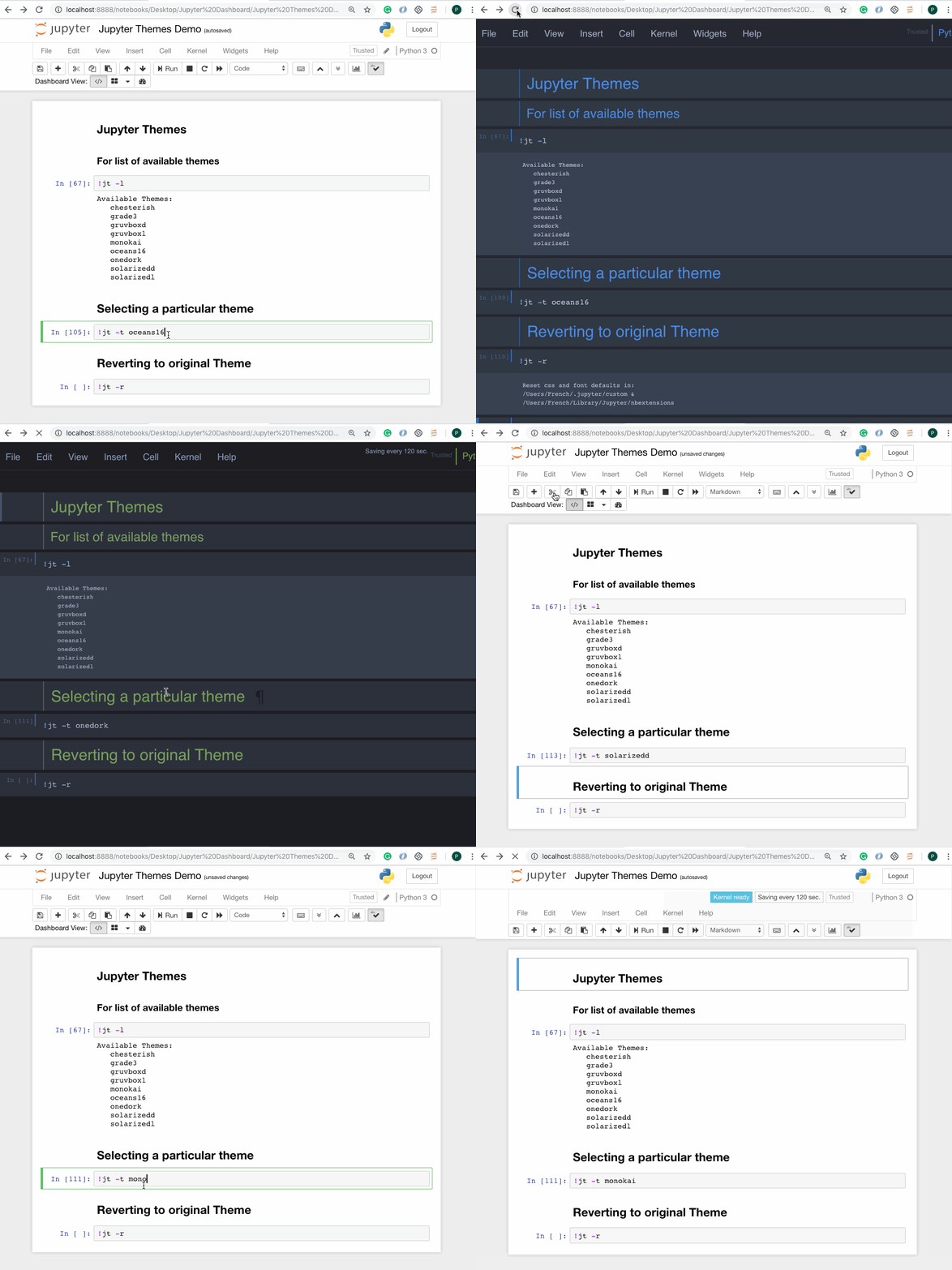
2. Jupyter Themes

pip install jupyterthemes
jt -l
# selecting a particular themejt -t <name of the theme># reverting to original Themejt -r
Left: original | Middle: Chesterish Theme | Right: solarizedl theme
Image for post

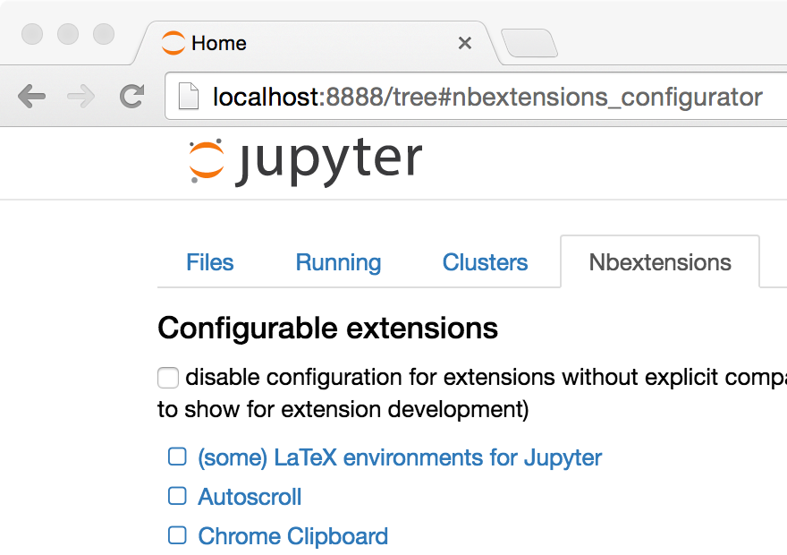
3. Notebook Extensions

Installation

conda install -c conda-forge jupyter_nbextensions_configurator
pip install jupyter_contrib_nbextensions && jupyter contrib nbextension install#incase you get permission errors on MacOS,pip install jupyter_contrib_nbextensions && jupyter contrib nbextension install --user
Image for post

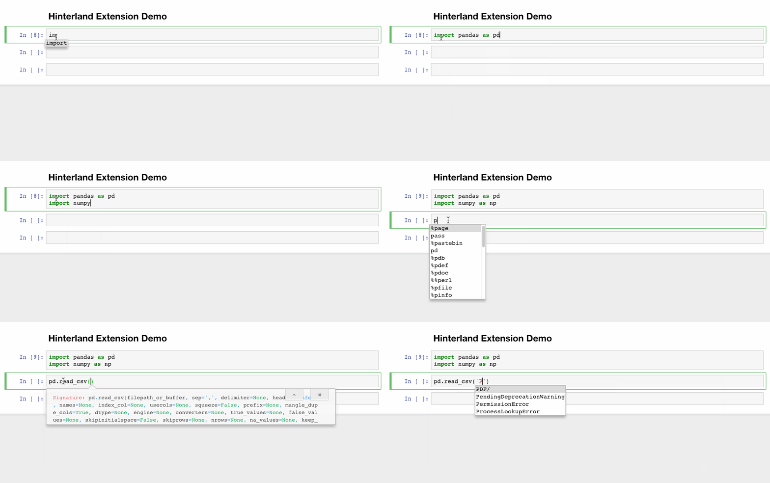
1. Hinterland

Image for post

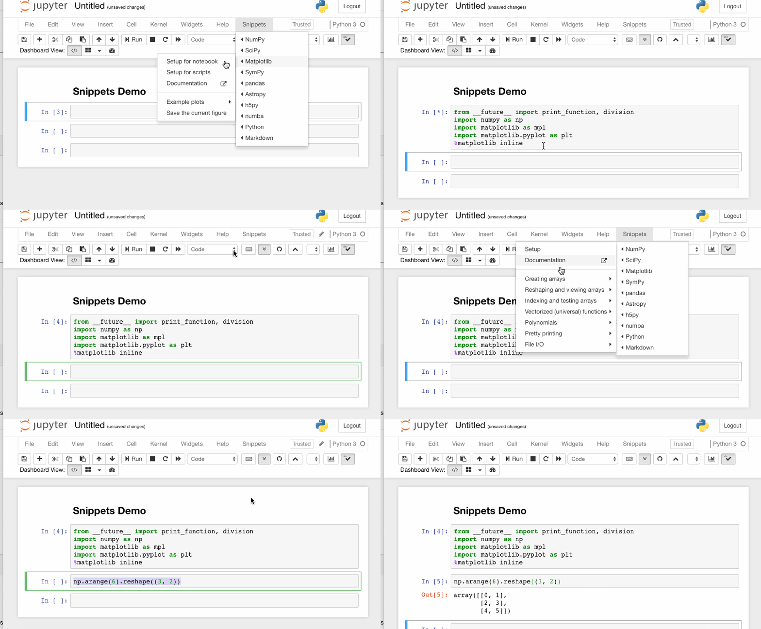
2. Snippets

Image for post

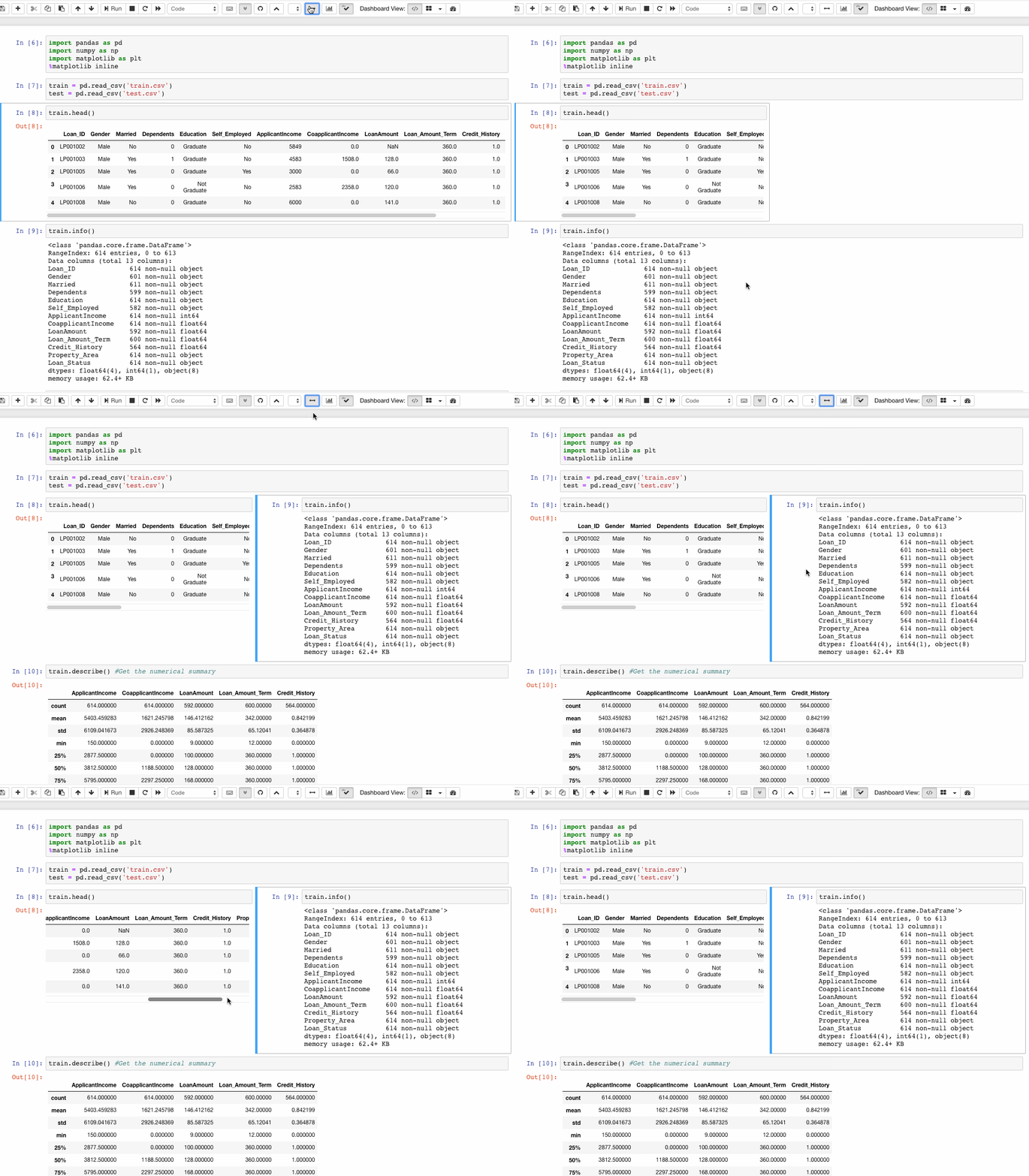
3. Split Cells Notebook

Image for post

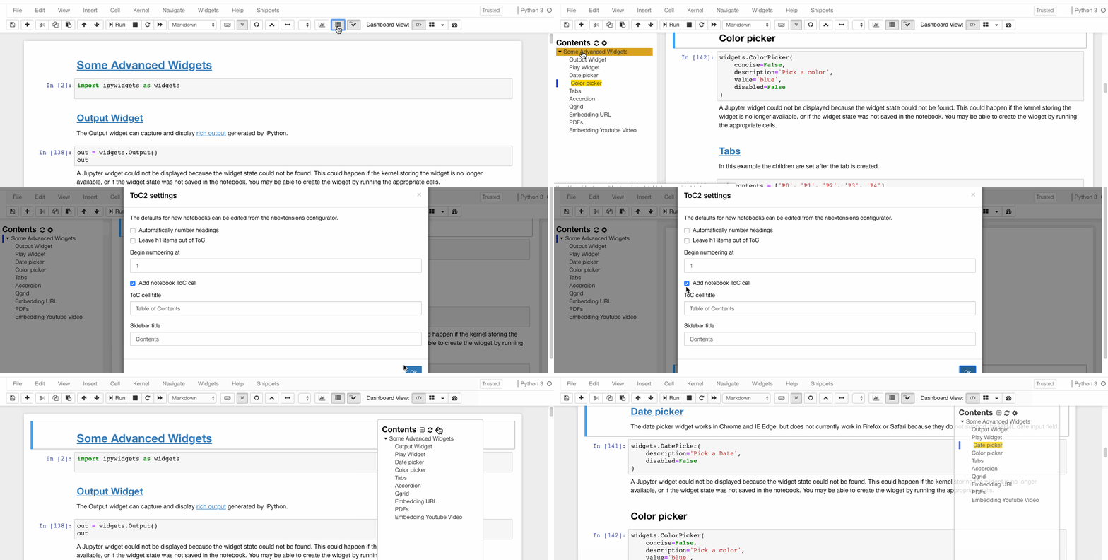
4. Table of Contents

Image for post

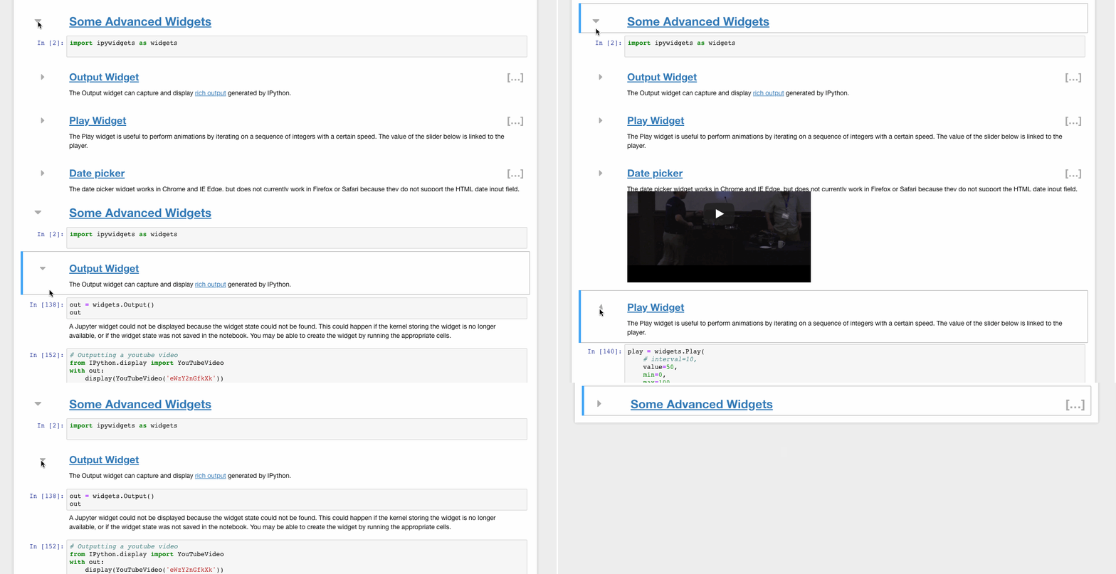
5. Collapsible Headings

Image for post

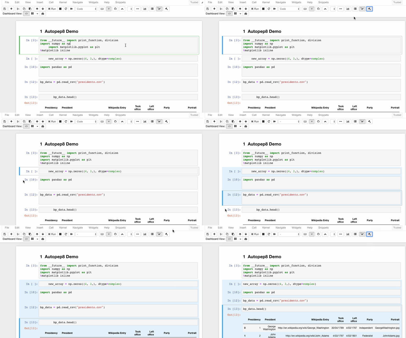
6. Autopep8

Image for post

4. Jupyter Widgets

Installation

# pip
pip install ipywidgets
jupyter nbextension enable --py widgetsnbextension
# Conda
conda install -c conda-forge ipywidgets
#Installing ipywidgets with conda automatically enables the extension
# Start with some imports!from ipywidgets import interact
import ipywidgets as widgets

1. Basic Widgets

def f(x):
return x
# Generate a slider
interact(f, x=10,);
Image for post
# Booleans generate check-boxes
interact(f, x=True);
Image for post
# Strings generate text areas
interact(f, x='Hi there!');
Image for post

2. Advanced Widgets

Play Widget

play = widgets.Play(
# interval=10,
value=50,
min=0,
max=100,
step=1,
description="Press play",
disabled=False
)
slider = widgets.IntSlider()
widgets.jslink((play, 'value'), (slider, 'value'))
widgets.HBox([play, slider])
Image for post

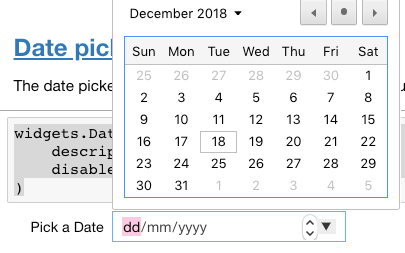
Date picker

widgets.DatePicker(
description='Pick a Date',
disabled=False
)
Image for post

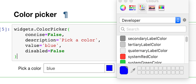
Color picker

widgets.ColorPicker(
concise=False,
description='Pick a color',
value='blue',
disabled=False
)
Image for post

Tabs

tab_contents = ['P0', 'P1', 'P2', 'P3', 'P4']
children = [widgets.Text(description=name) for name in tab_contents]
tab = widgets.Tab()
tab.children = children
for i in range(len(children)):
tab.set_title(i, str(i))
tab
Image for post

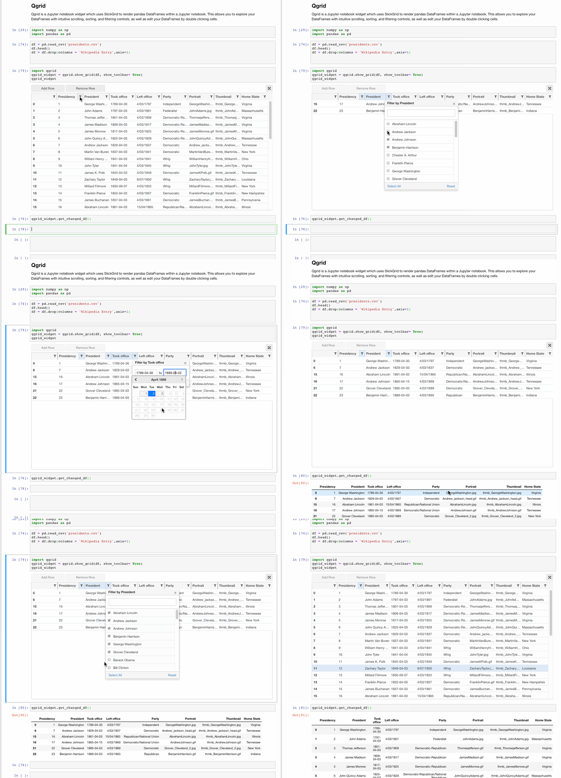
5. Qgrid

Installation

pip install qgrid
jupyter nbextension enable --py --sys-prefix qgrid
# only required if you have not enabled the ipywidgets nbextension yet
jupyter nbextension enable --py --sys-prefix widgetsnbextension
# only required if you have not added conda-forge to your channels yet
conda config --add channels conda-forge
conda install qgrid
Image for post

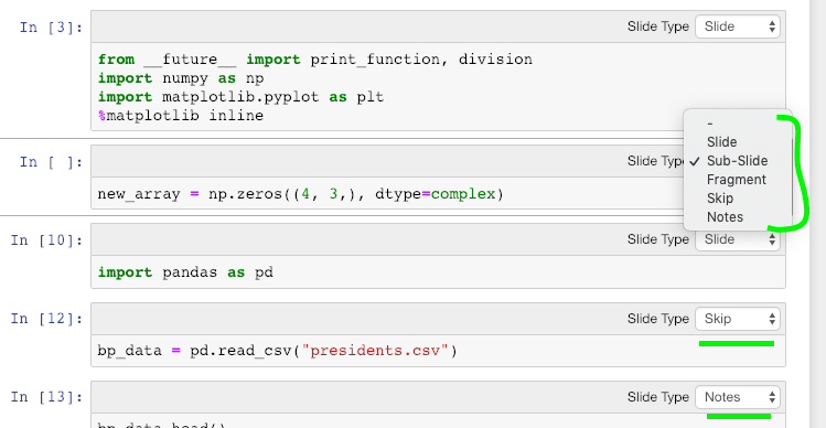
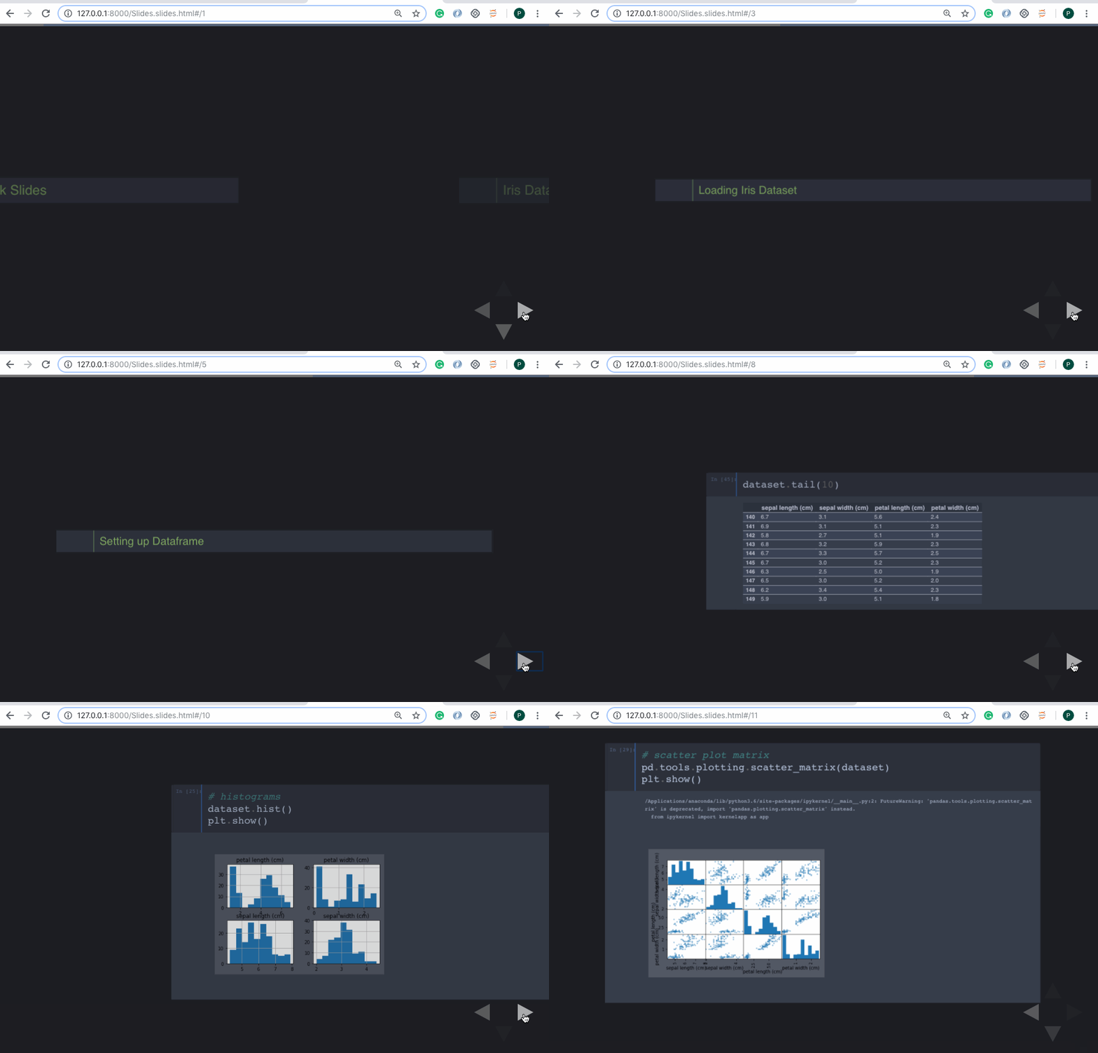
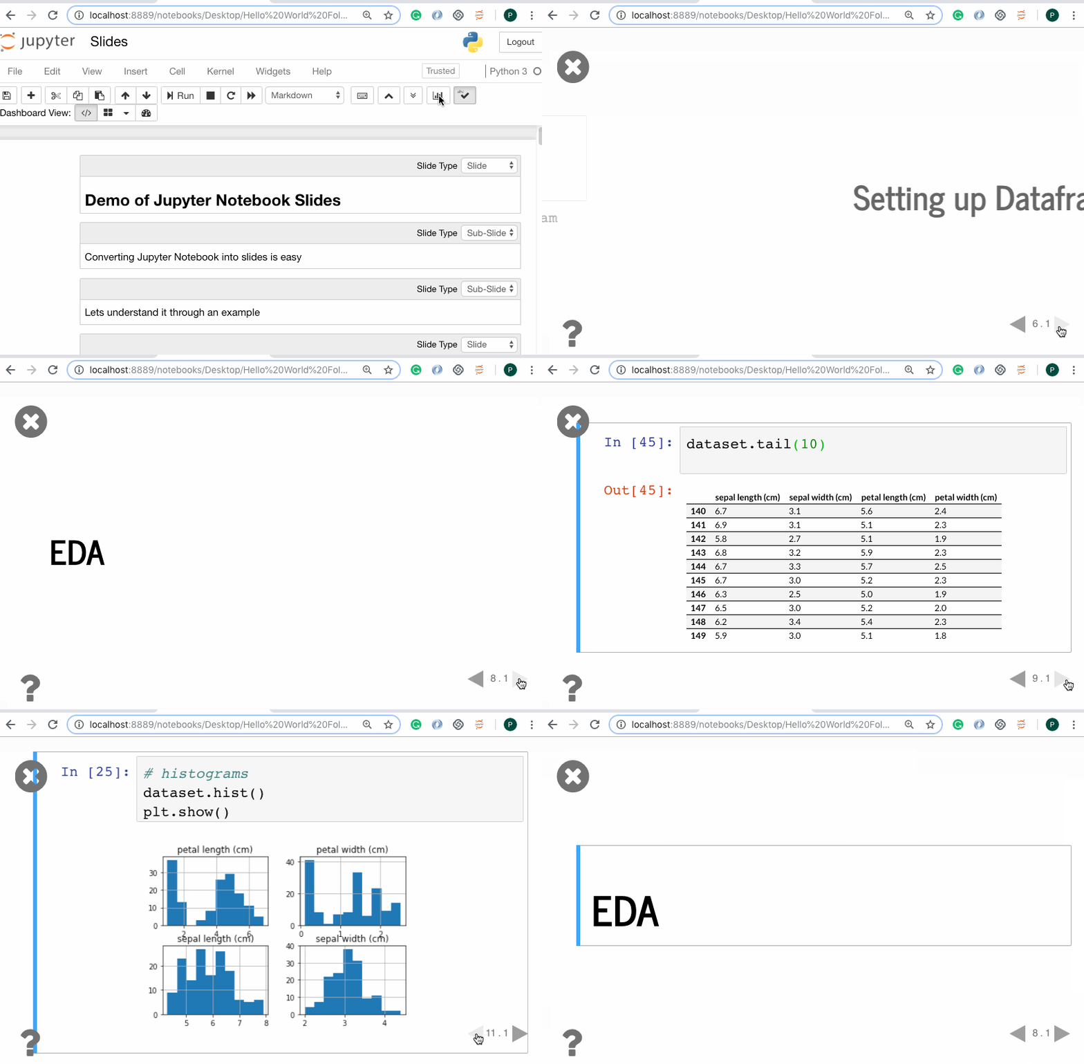
6. Slideshow

1. Jupyter Notebook’s built-in Slide option

Image for post
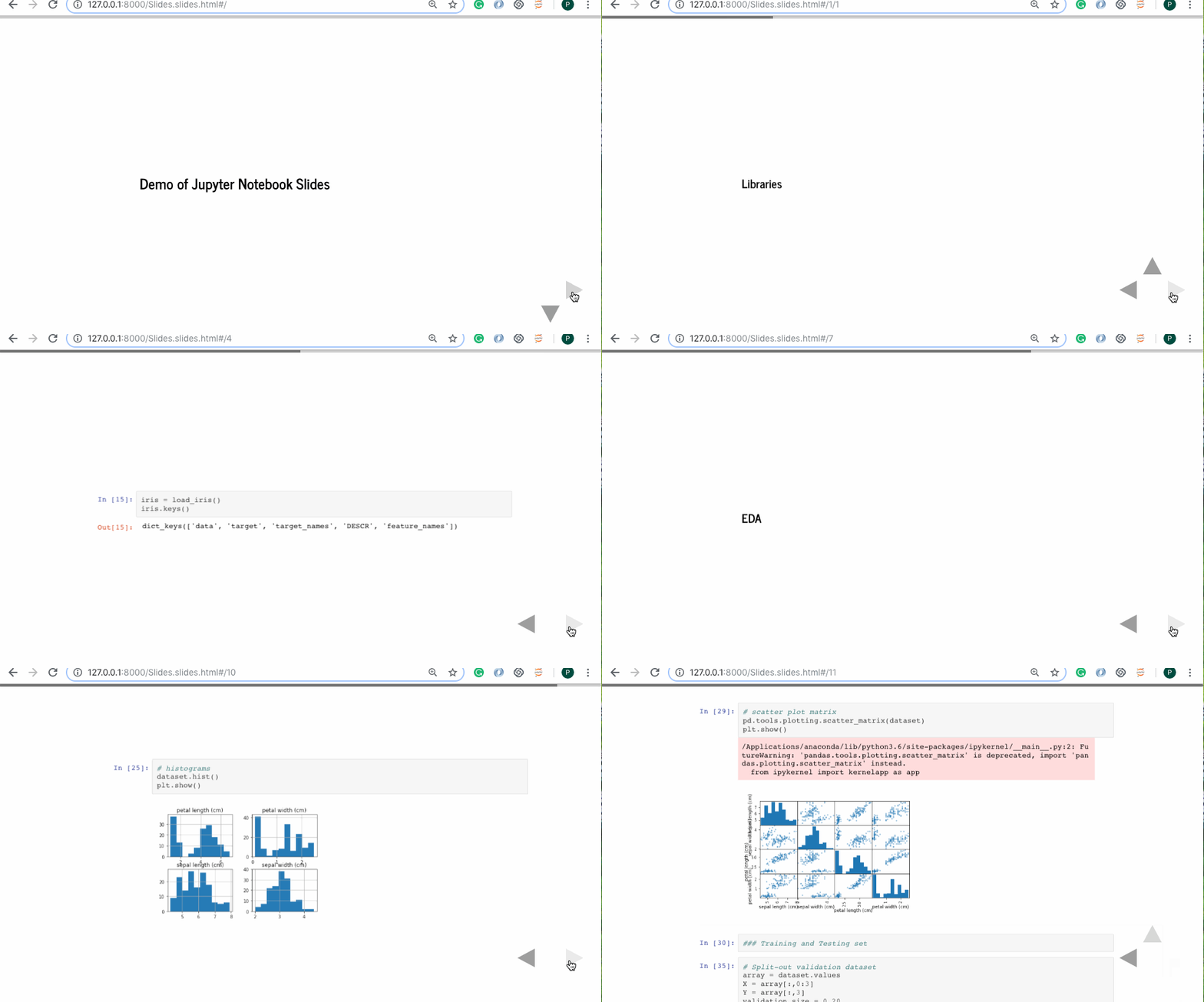
jupyter nbconvert *.ipynb --to slides --post serve
# insert your notebook name instead of *.ipynb
Image for post
Image for post

2. Using the RISE plugin

conda install -c damianavila82 rise
pip install RISE
jupyter-nbextension install rise --py --sys-prefix#enable the nbextension:
jupyter-nbextension enable rise --py --sys-prefix
Image for post
Image for post

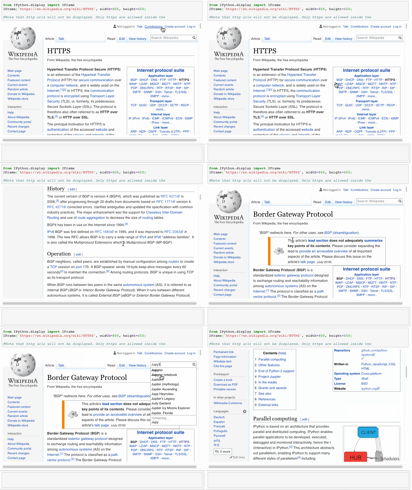
6. Embedding URLs, PDFs, and Youtube Videos

URLs

#Note that http urls will not be displayed. Only https are allowed inside the Iframefrom IPython.display import IFrame
IFrame('https://en.wikipedia.org/wiki/HTTPS', width=800, height=450)
Image for post

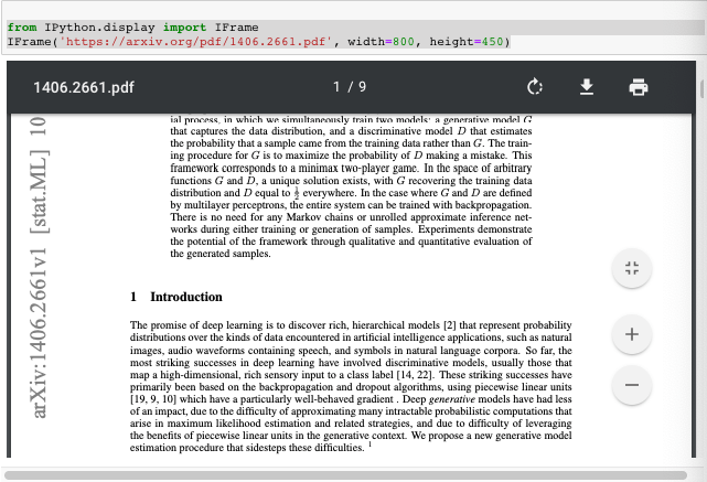
PDFs

from IPython.display import IFrame
IFrame('https://arxiv.org/pdf/1406.2661.pdf', width=800, height=450)
Image for post

Youtube Videos

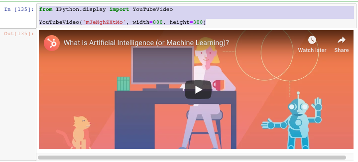
from IPython.display import YouTubeVideoYouTubeVideo('mJeNghZXtMo', width=800, height=300)
Image for post

Conclusion

Please Stop Doing These 5 Things in Pandas

These mistakes are super common and super easy to fix.

As someone who did over a decade of development before moving into Data Science, there’s a lot of mistakes I see data scientists make while using Pandas. The good news is these are really easy to avoid, and fixing them can also make your code more readable.

Image for post
Photo by Daniela Holzer on Unsplash

Mistake 1: Getting or Setting Values Slowly

It’s nobody’s fault that there are way too many ways to get and set values in Pandas. In some situations, you have to find a value using only an index or find the index using only the value. However, in many cases, you’ll have many different ways of selecting data at your disposal: index, value, label, etc.

In those situations, I prefer to use whatever is fastest. Here are some common choices from slowest to fastest, which shows you could be missing out on a 195% gain!

Tests were run using a DataFrame of 20,000 rows. Here’s the notebook if you want to run it yourself.

# .at - 22.3 seconds
for i in range(df_size):
df.at[i] = profile
Wall time: 22.3 s
# .iloc - 15% faster than .at
for i in range(df_size):
df.iloc[i] = profile
Wall time: 19.1 s
# .loc - 30% faster than .at
for i in range(df_size):
df.loc[i] = profile
Wall time: 16.5 s
# .iat, doesn't work for replacing multiple columns of data.
# Fast but isn't comparable since I'm only replacing one column.
for i in range(df_size):
df.iloc[i].iat[0] = profile['address']
Wall time: 3.46 s
# .values / .to_numpy() - 195% faster than .at
for i in range(df_size):
df.values[i] = profile
# Recommend using to_numpy() instead if you have Pandas 1.0+
# df.to_numpy()[i] = profile
Wall time: 254 ms

(As Alex Bruening and miraculixx noted in the comments, for loops are not the ideal way to perform actions like this, look at .apply(). I’m using them here purely to prove the speed difference of the line inside the loop.)

Mistake 2: Only Using 25% of Your CPU

Whether you’re on a server or just your laptop, the vast majority of people never use all the computing power they have. Most processors (CPUs) have 4 cores nowadays, and by default, Pandas will only ever use one.

From the Modin Docs, a 4x speedup on a 4 core machine.

Modin is a Python module built to enhance Pandas by making way better use of your hardware. Modin DataFrames don’t require any extra code and in most cases will speed up everything you do to DataFrames by 3x or more.

Modin acts as more of a plugin than a library since it uses Pandas as a fallback and cannot be used on its own.

The goal of Modin is to augment Pandas quietly and let you keep working without learning a new library. The only line of code most people will need is import modin.pandas as pd replacing your normal import pandas as pd, but if you want to learn more check out the documentation here.

In order to avoid recreating tests that have already been done, I’ve included this picture from the Modin documentation showing how much it can speed up the read_csv() function on a standard laptop.

Please note that Modin is in development, and while I use it in production, you should expect some bugs. Check the Issues in GitHub and the Supported APIs for more information.

Mistake 3: Making Pandas Guess Data Types

When you import data into a DataFrame and don’t specifically tell Pandas the columns and datatypes, Pandas will read the entire dataset into memory just to figure out the data types.

For example, if you have a column full of text Pandas will read every value, see that they’re all strings, and set the data type to “string” for that column. Then it repeats this process for all your other columns.

You can use df.info() to see how much memory a DataFrame uses, that’s roughly the same amount of memory Pandas will consume just to figure out the data types of each column.

Unless you’re tossing around tiny datasets or your columns are changing constantly, you should always specify the data types. In order to do this, just add the dtypes parameter and a dictionary with your column names and their data types as strings. For example:

pd.read_csv(‘fake_profiles.csv’, dtype={
‘job’: ‘str’,
‘company’: ‘str’,
‘ssn’: ‘str’
})

Note: This also applies to DataFrames that don’t come from CSVs.

Mistake 4: Leftover DataFrames

One of the best qualities of DataFrames is how easy they are to create and change. The unfortunate side effect of this is most people end up with code like this:

# Change dataframe 1 and save it into a new dataframedf1 = pd.read_csv(‘file.csv’)df2 = df1.dropna()df3 = df2.groupby(‘thing’)

What happens is you leave df2 and df1 in Python memory, even though you’ve moved on to df3. Don’t leave extra DataFrames sitting around in memory, if you’re using a laptop it’s hurting the performance of almost everything you do. If you’re on a server, it’s hurting the performance of everyone else on that server (or at some point, you’ll get an “out of memory” error).

Instead, here are some easy ways to keep your memory clean:

  • Use df.info() to see how much memory a DataFrame is using
  • Install plugin support in Jupyter, then install the Variable Inspector plugin for Jupyter. If you’re used to having a variable inspector in R-Studio, you should know that R-Studio now supports Python!
  • If you’re in a Jupyter session already, you can always erase variables without restarting by using del df2
  • Chain together multiple DataFrame modifications in one line (so long as it doesn’t make your code unreadable): df = df.apply(thing1).dropna()
  • As Roberto Bruno Martins pointed out, another way to ensure clean memory is to perform operations within functions. You can still unintentionally abuse memory this way, and explaining scope is outside the scope of this article, but if you aren’t familiar I’d encourage you to read this writeup.

Mistake 5: Manually Configuring Matplotlib

This might be the most common mistake, but it lands at #5 because it’s the least impactful. I see this mistake happen even in tutorials and blog posts from experienced professionals.

Matplotlib is automatically imported by Pandas, and it even sets some chart configuration up for you on every DataFrame.

There’s no need to import and configure it for every chart when it’s already baked into Pandas for you.

Here’s an example of doing it the wrong way, even though this is a basic chart it’s still a waste of code:

import matplotlib.pyplot as plt
ax.hist(x=df[‘x’])
ax.set_xlabel(‘label for column X’)
plt.show()

And here’s the right way:

df[‘x’].plot()

Easier, right? You can do anything on these DataFrame plot objects that you can do to any other Matplotlib plot object. For example:

df[‘x’].plot.hist(title=’Chart title’)

I’m sure I’m making other mistakes I don’t know about, but hopefully sharing these known ones with you will help put your hardware to better use, let you write less code, and get more done!

If you’re still looking for more optimizations, you’ll definitely want to read:

Interactive spreadsheets in Jupyter

Image for post

ipywidgets plays an essential part in the Jupyter ecosystem; it brings interactivity between user and data.

Widgets are eventful Python objects that often have a visual representation in the Jupyter Notebook or JupyterLab: a button, a slider, a text input, a checkbox…

More than a library of interactive widgets, ipywidgets is a powerful framework upon which it is straightforward to create new custom widgets. Developers can quickly start their own widgets library with best practices of code structure and packaging using the widget-cookiecutter project.

You can find examples of really nice widgets libraries in the blog-post: Video streaming in the Jupyter Notebook.


A spreadsheet is an interactive tool for data analysis in a tabular form. It consists of cells and cell ranges. It supports value dependent cell formatting/styling and one can apply mathematical functions on cells and perform chained computations. It is the perfect user interface for statistical and financial operations.

The Jupyter Notebook was lacking a spreadsheet library, that’s when ipysheet comes into play.

ipysheet

ipysheet is a new interactive widgets library that aims at implementing the core features of a good spreadsheet application and more.

There are two main widgets in ipysheet, the Cell widget, and the Sheet widget. We provide helper functions for creating rows, columns and cell ranges in general.

The cell value can be a boolean, a numerical value, a string, a date, and of course another widget!

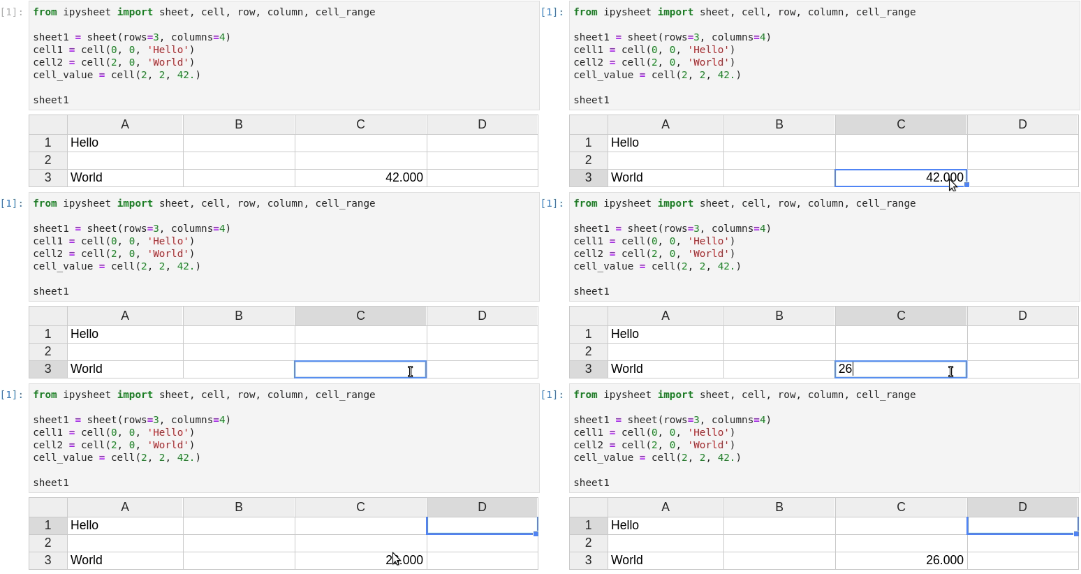
ipysheet uses a Matplotlib-like API for creating a sheet:

Image for post

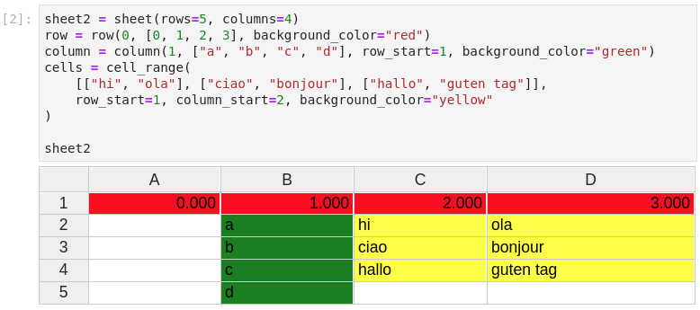
The user can create entire rows, columns, and even cell ranges:

Image for post

Of course, values in cells are dynamic, the cell value can be dynamically updated from Python and the new value will be visible in the sheet.

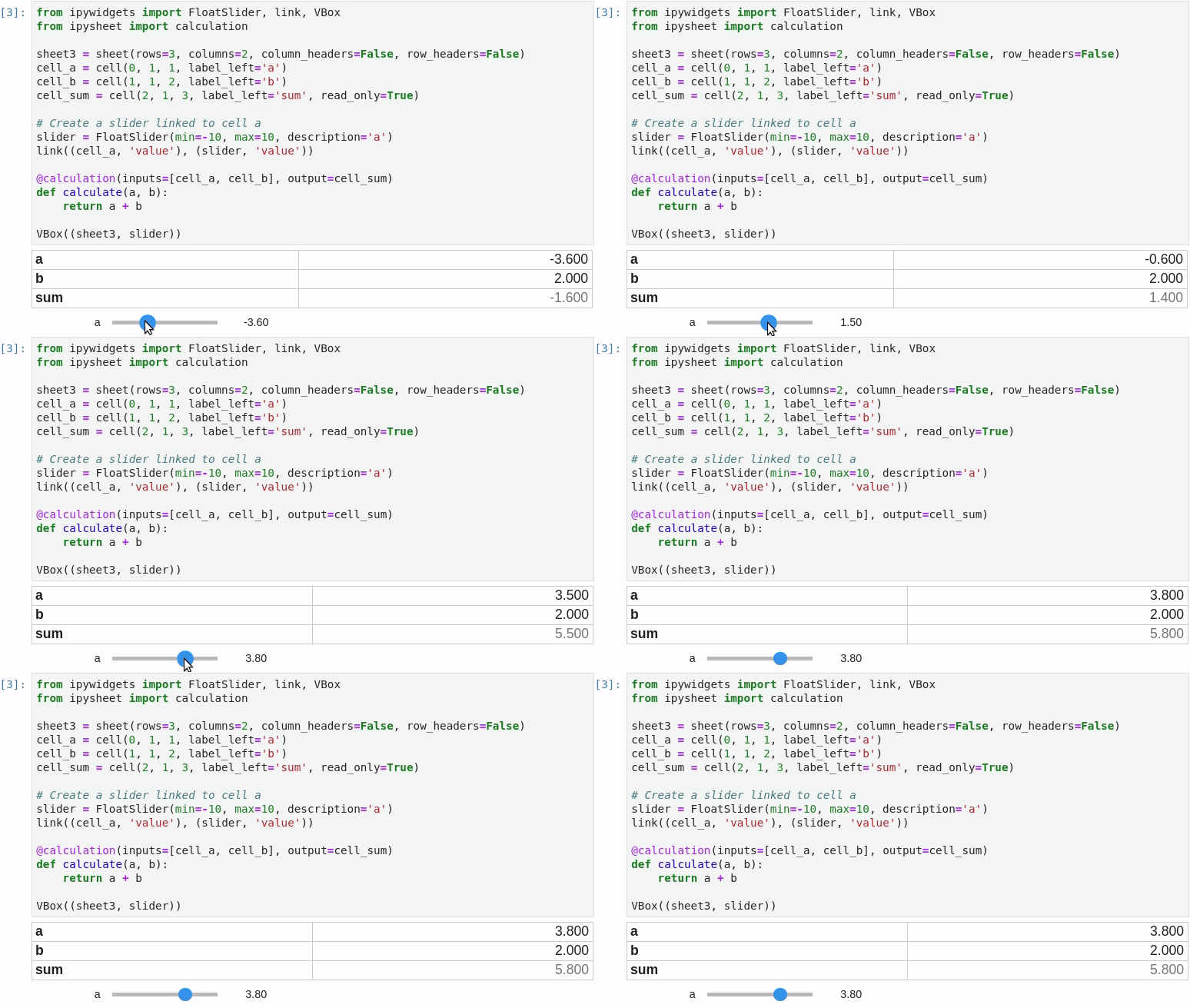
It is possible to link a cell value to a widget (in the following screenshot a FloatSlider widget is linked to cell “a”) and to define a specific cell as the result of a custom calculation depending on other cells:

Image for post

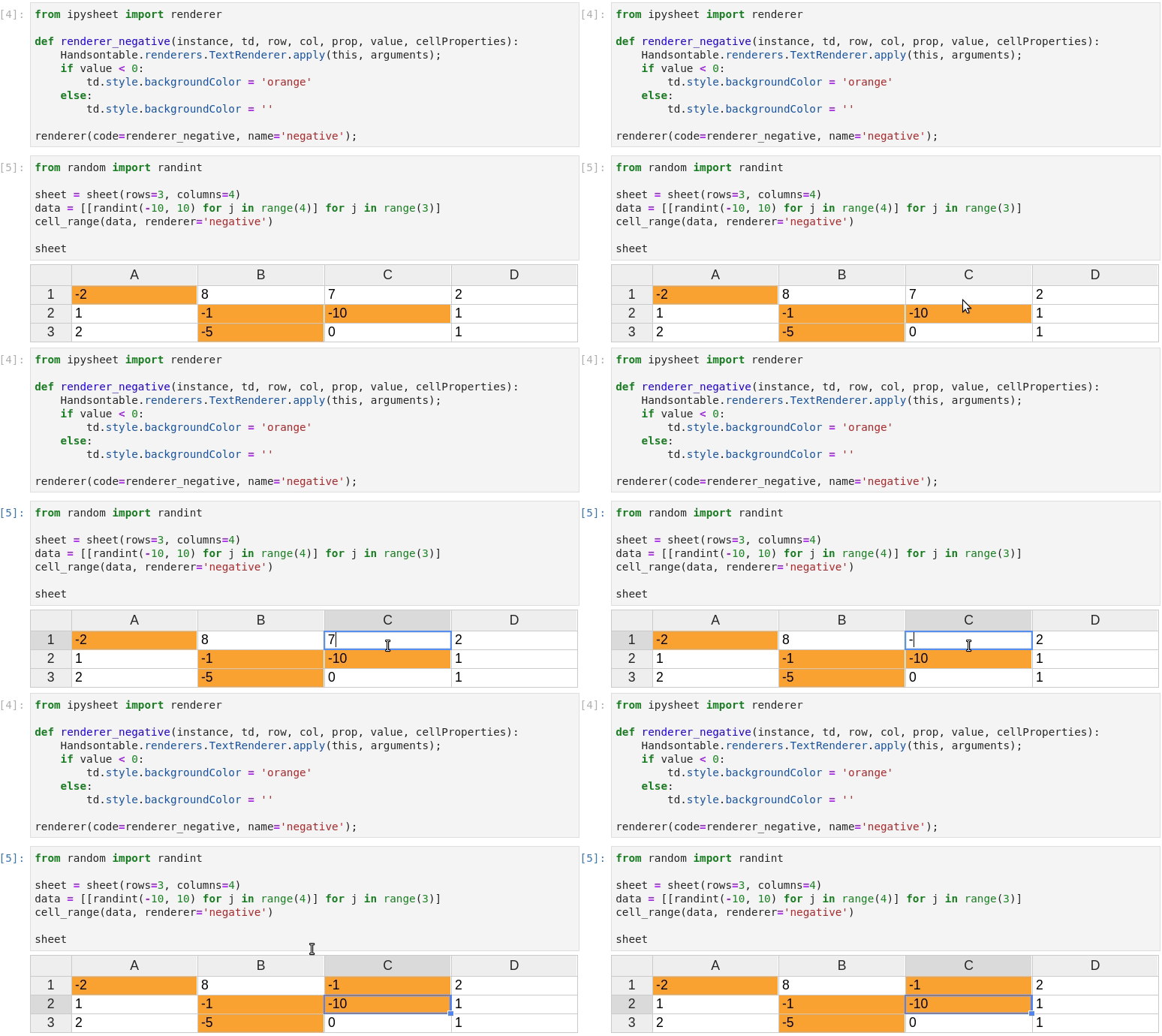
Custom styling can be used, using what we call renderers:

Image for post

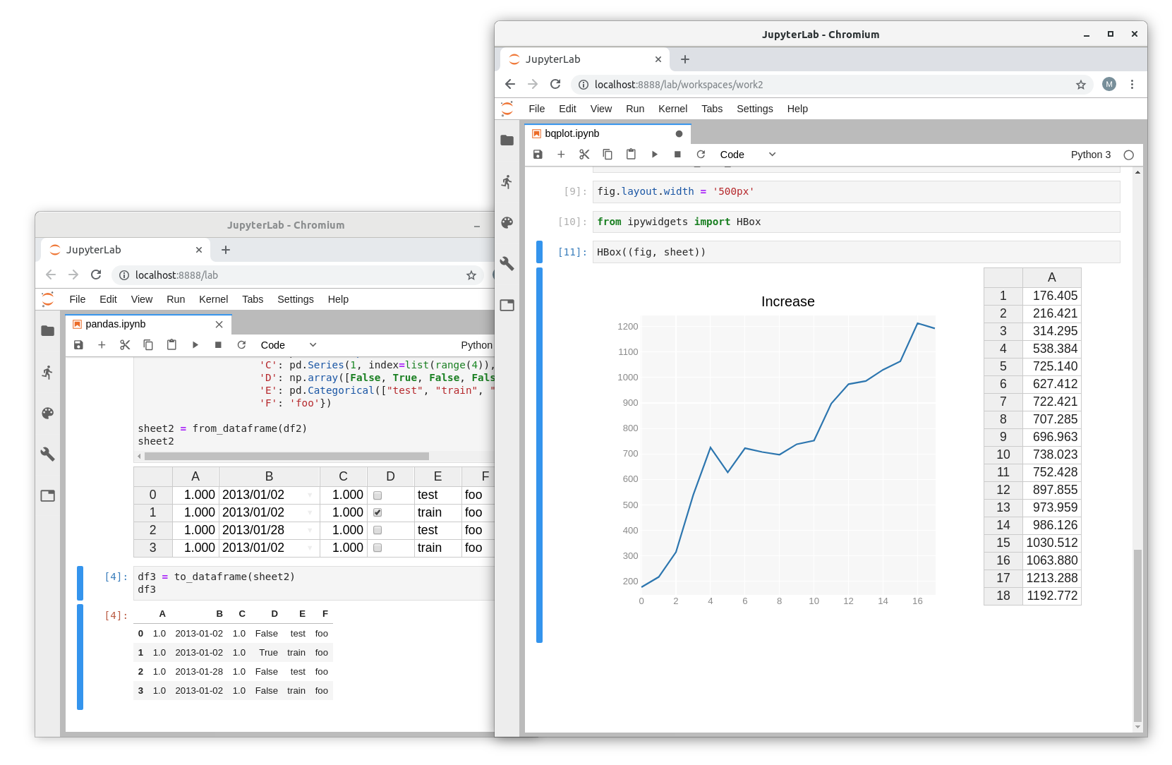
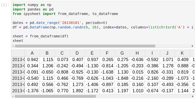
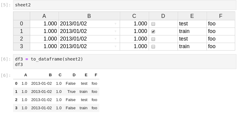
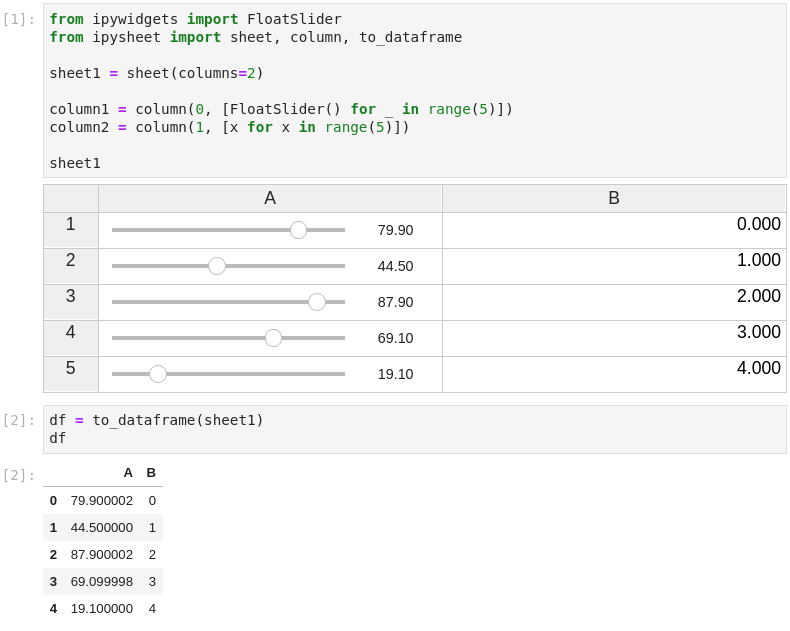
Adding support to NumPy Arrays and Pandas Dataframes loading and exporting was an important feature that we wanted. ipysheet provides from_array, to_array, from_dataframe and to_dataframe functions for this purpose:

Image for post
Image for post

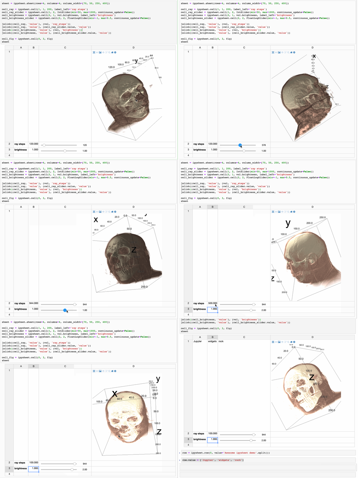
Another killer feature is that a cell value can be ANY interactive widget. This means that the user can put a button or a slider widget in a cell:

Image for post

But it also means that a higher level widget can be put in a cell. Whether the widget is a plot from bqplot, a map from ipyleaflet or even a multi-volume rendering from ipyvolume:

Image for post

You can try it right now with binder, without the need of installing anything on your computer, just by clicking on this button:

Image for post

The source code is hosted on Github: https://github.com/QuantStack/ipysheet/

Similar projects

Acknowledgments

The development of ipysheet is led by QuantStack.

Image for post

This development is sponsored by Société Générale and Bloomberg.

About the Authors

Maarten Breddels is an entrepreneur and freelance developer / consultant / data scientist working mostly with Python, C++ and Javascript in the Jupyter ecosystem. Founder of vaex.io. His expertise ranges from fast numerical computation, API design, to 3d visualization. He has a Bachelor in ICT, a Master and PhD in Astronomy, likes to code and solve problems.


Martin Renou is a Scientific Software Engineer at QuantStack. Before joining QuantStack, he studied at the French Aerospace Engineering School SUPAERO. He also worked at Logilab in Paris and Enthought in Cambridge. As an open source developer at QuantStack, Martin worked on a variety of projects, from xsimd, xtensor, xframe, xeus and xeus-python in C++ to ipyleaflet and ipywebrtc in Python and JavaScript.

Pandas DataFrame (Python): 10 useful tricks

10 basic tricks to make your pandas life a bit easier

Image for post

Pandas is a powerful open source data analysis and manipulation tool, built on top of the Python programming language. In this article, I will show 10 tricks regarding the pandas DataFrame to make certain programming practices a bit easier.

Of course, before we can use pandas, we have to import it by using the following command:

import pandas as pd

1. Select multiple rows and columns using .loc

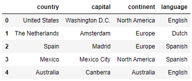
countries = pd.DataFrame({
'country': ['United States', 'The Netherlands', 'Spain', 'Mexico', 'Australia'],
'capital': ['Washington D.C.', 'Amsterdam', 'Madrid', 'Mexico City', 'Canberra'],
'continent': ['North America', 'Europe', 'Europe', 'North America', 'Australia'],
'language': ['English', 'Dutch', 'Spanish', 'Spanish', 'English']})
Image for post

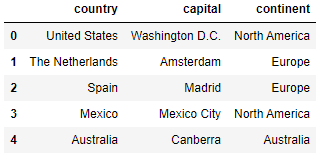
By using the operator, we are able to select subsets of rows and columns on the basis of their index label and column name. Below are some examples on how to use the loc operator on the ‘countries’ DataFrame:

countries.loc[:, 'country':'continent']
Image for post
countries.loc[0:2, 'country':'continent']
Image for post
countries.loc[[0, 4], ['country', 'language']]
Image for post

2. Filter DataFrames by category

In many cases, we may want to consider only the data points that are included in one particular category, or sometimes in a selection of categories. For a single category, we are able to do this by using the operator. However, for multiple categories, we have to make use of the function:

countries[countries.continent == 'Europe']
Image for post
countries[countries.language.isin(['Dutch', 'English'])]
Image for post

3. Filter DataFrames by excluding categories

As opposed to filtering by category, we may want to filter our DataFrame by excluding certain categories. We do this by making use of the (tilde) sign, which is the complement operator. Example usage:

countries[~countries.continent.isin(['Europe'])]
Image for post
countries[~countries.language.isin(['Dutch', 'English'])]
Image for post

4. Rename columns

You might want to change the name of certain columns because e.g. the name is incorrect or incomplete. For example, we might want to change the ‘capital’ column name to ‘capital_city’ and ‘language’ to ‘most_spoken_language’. We can do this in the following way:

countries.rename({'capital': 'capital_city', 'language': 'most_spoken_language'}, axis='columns')
Image for post

Alternatively, we can use:

countries.columns = ['country', 'capital_city', 'continent', 'most_spoken_language']

5. Reverse row order

To reverse the row order, we make use of the operator. This works in the following way:

countries.loc[::-1]
Image for post

However, note that now the indexes still are following the previous ordering. We have to make use of the function to reset the indexes:

countries.loc[::-1].reset_index(drop=True)
Image for post

6. Reverse column order

Reversing the column order goes in a similar way as for the rows:

countries.loc[:, ::-1]
Image for post

7. Split a DataFrame into two random subsets

In some cases, we want to split a DataFrame into two random subsets. For this, we make use of the function. For example, when creating a training and a test set out of the whole data set, we have to create two random subsets. Below, we show how to use the function:

countries_1 = countries.sample(frac=0.6, random_state=999)
countries_2 = countries.drop(countries_1.index)
Image for post
countries_1
Image for post
countries_2

8. Create dummy variables

students = pd.DataFrame({
'name': ['Ben', 'Tina', 'John', 'Eric'],
'gender': ['male', 'female', 'male', 'male']})

We might want to convert categorical variables into dummy/indicator variables. We can do so by making use of the function:

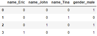
pd.get_dummies(students)
Image for post

To get rid of the redundant columns, we have to add :

pd.get_dummies(students, drop_first=True)
Image for post

9. Check equality of columns

When the goal is to check equality of two different columns, one might at first think of the operator, since this is mostly used when we are concerned with checking equality conditions. However, this operator does not handle NaN values properly, so we make use of the functions here. This goes as follows:

df = pd.DataFrame({'col_1': [1, 0], 'col_2': [0, 1], 'col_3': [1, 0]})
Image for post
df['col_1'].equals(df['col_2'])

>>> False

df['col_1'].equals(df['col_3'])

>>> True

10. Concatenate DataFrames

We might want to combine two DataFrames into one DataFrame that contains all data points. This can be achieved by using the function:

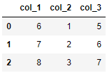
df_1 = pd.DataFrame({'col_1': [6, 7, 8], 'col_2': [1, 2, 3], 'col_3': [5, 6, 7]})
Image for post
pd.concat([df, df_1]).reset_index(drop=True)

Thanks for reading!

I hope this article helped you in some way, and I wish you good luck on your next project when making use of Pandas :).

Introducing Bamboolib — a GUI for Pandas

A couple of days back, mister Tobias Krabel contacted me via LinkedIn to introduce me to his product, a Python library called Bamboolib, which he states to be a GUI tool for learning Pandas — Python’s data analysis and visualization library.

He states, and I quote:

I have to admit, I was skeptical at first, mainly because I’m not a big fan of GUI tools and drag & drop principle in general. Still, I’ve opened the URL and watched the introduction video.

It was one of those rare times when I was legitimately intrigued.

From there I’ve quickly responded to Tobias, and he kindly offered me to test out the library and see if I liked it.

How was it? Well, you’ll have to keep reading to find the answer to that. So let’s get started.


Is it Free?

In a world where such amazing libraries like Numpy and Pandas are free to use, this question may not even pop in your head. However, it should, because not all versions of Bamboolib are free.

If you don’t mind sharing your work with others, then yeah, it’s free to use, but if that poses a problem then it will set you back at least $10 a month which might be a bummer for the average users. Down below is the full pricing list:

Image for post

As the developer of the library stated, Bamboolib is designed to help you learn Pandas, so I don’t see a problem with going with the free option — most likely you won’t be working on some top-secret project if just starting out.

This review will, however, be based on the private version of the library, as that’s the one Tobias gave access to me. With that being said, this article is by no means written with the idea of persuading you to buy the license, it only provides my personal opinion.

Before jumping into the good stuff, you’ll need to install the library first.


The Installation Process

The first and most obvious thing to do is pip install:

pip install bamboolib

However, there’s a lot more to do if you want this thing fully working. It is designed to be a Jupyter Lab extension (or Jupyter Notebook if you still use those), so we’ll need to set up a couple of things there also.

In a command line type the following:

jupyter nbextension enable --py qgrid --sys-prefix
jupyter nbextension enable --py widgetsnbextension --sys-prefix
jupyter nbextension install --py bamboolib --sys-prefix
jupyter nbextension enable --py bamboolib --sys-prefix

Now you’ll need to find the major version of Jupyter Lab installed on your machine. You can obtain it with the following command:

jupyter labextension list

Mine is “1.0”, but yours can be anything, so here’s a generic version of the next command you’ll need to execute:

jupyter labextension install @jupyter-widgets/jupyterlab-manager@MAJOR_VERSION.MINOR_VERSION --no-build

Note that you need to replace “MAJOR_VERSION.MINOR_VERSION” with the version number, which is “1.0” in my case.

A couple of commands more and you’re ready to rock:

jupyter labextension install @8080labs/qgrid@1.1.1 --no-build
jupyter labextension install plotlywidget --no-build
jupyter labextension install jupyterlab-plotly --no-build
jupyter labextension install bamboolib --no-build

jupyter lab build --minimize=False

That’ it. Now you can start Juypter Lab and we can dive into the good stuff.


The First Use

Once in Jupyter, you can import Bamboolib and Pandas, and then use Pandas to load in some dataset:

Image for post

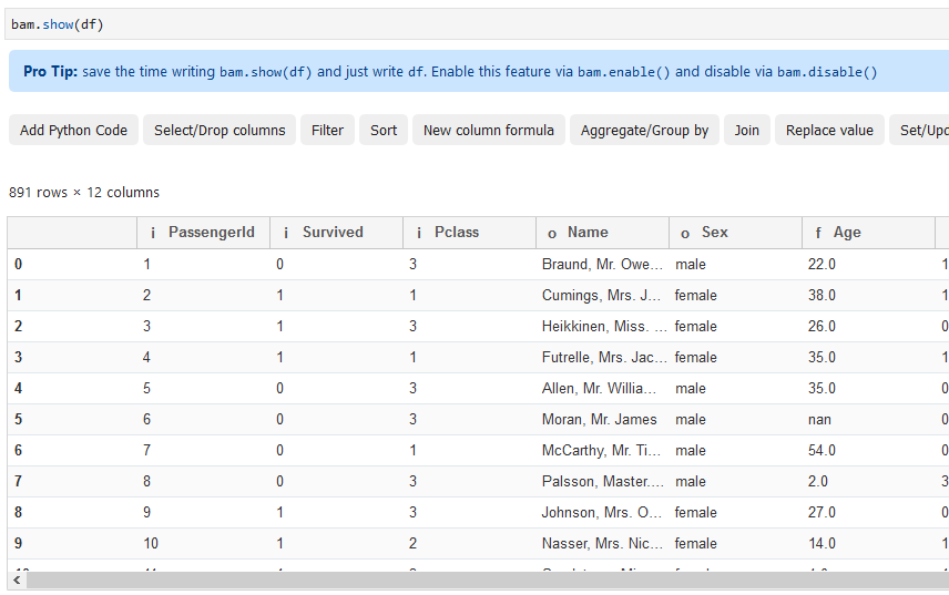
Here’s how you’d use the library to view the dataset:

Image for post

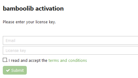
That’s not gonna work the first time you’re using the library. You’ll need to activate it, so make sure to have the license key somewhere near:

Image for post

Once you’ve entered the email and license key, you should get the following message indicating that everything went well:

Image for post

Great, now you can once again execute the previous cell. Immediately you’ll see an unfamiliar, but friendly-looking interface:

Image for post

Now everything is good to go, and we can dive into some basic functionalities. It was a lot of work to get to this point, but trust me, it was worth it!


Data Filtering

One of the most common everyday tasks of any data analyst/scientist is data filtering. Basically you want to keep only a subset of data that’s relevant to you in a given moment.

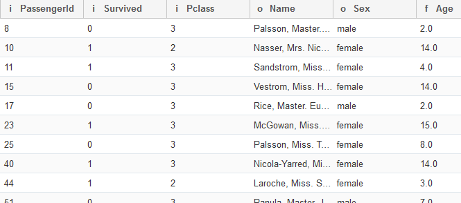
To start filtering with Bamboolib, click on the Filter button.

A side menu like the one below should pop up. I’ve decided to filter by the “Age” column, and keep only the rows where the value of “Age” is less than 18:

Image for post

Once you press Execute, you’ll see the actions took place immediately:

Image for post

That’s great! But what more can you do?


Replacing Values

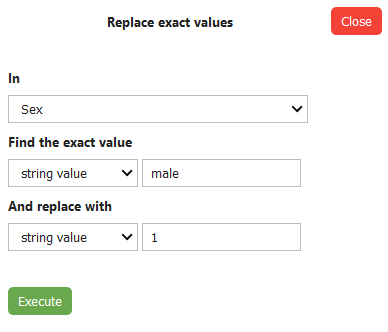
Another one of those common everyday tasks is to replace string values with the respective numerical alternative. This dataset is perfect to demonstrate value replacement because we can easily replace string values in the “Sex” column with numeric ones.

To begin, hit the Replace value button and specify the column, the value you want to replace and what you want to replace it with:

Image for post

And once the Execute button is hit:

Fantastic! You can do the same for the “female” option, but it’s up to you whether you want to do it or not.


Group By

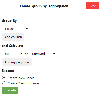
Yes, you can also perform aggregations! To get started, click on the Aggregate/Group by button and specify what should be done in the side menu.

I’ve decided to group by “Pclass”, because I want to see the total number of survivors per passenger class:

Image for post

That will yield the following output:

Image for post

Awesome! Let’s explore one more thing before wrapping up.


One Hot Encoding

Many times when preparing data for machine learning you’ll want to create dummy variables, ergo create a new column per unique value of a given attribute. It’s a good idea to do so because many machine learning algorithms can’t work with text data.

To implement that logic via Bamboolib, hit the OneHotEncoder button. I’ve decided to create dummy variables from the “Embarked” attribute because it has 3 distinct values and you can’t state that one is better than the other. Also, make sure to remove the first dummy to avoid collinearity issues (having variable which is a perfect predictor for some other variable):

Image for post

Executing will create two new columns in the dataset, just as you would expect:

That’s nice, I’ve done my transformations, but what’s next?


Getting the Code

It was all fun and games until now, but sooner or later you’ll notice the operations don’t act in place — ergo the dataset will not get modified if you don’t explicitly specify it.

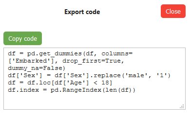
That’s not a bug, as it enables you to play around without messing the original dataset. What Bamboolib will do, however, it will generate Python code for achieving the desired transformations.

To get the code, first, click on the Export button:

Image for post

Now specify how do you want it exported — I’ve selected the first option:

Image for post

And it will finally give you the code which you can copy and apply to the dataset:

Image for post

Is it worth it?

Until this point, I showcased briefly the main functionalities of Bamboolib — by no means was it exhaustive tutorial — just wanted to show you the idea behind it.

The question remains, is it worth the money?

That is if you decide to go with the paid route. You can still use it for free, provided that you don’t mind sharing your work with others. The library by itself is worth checking out for two main reasons:

  1. It provides a great way to learn Pandas — it’s much more easy to learn by doing than by reading, and a GUI tool like this will most certainly only help you
  2. It’s great for playing around with data — let’s face it, there are times when you know what you want to do, but you just don’t know how to implement it in code — Bamboolib can assist

Keep in mind — you won’t get any additional features with the paid version — the only real benefit is that your work will be private and that there’s an option for commercial use.

Even if you’re not ready to grab your credit card just yet, it can’t harm you to try out the free version and see if it’s something you can benefit from.

Thanks for reading. Take care.

Jupyter is now a full-fledged IDE

Literate programming is now a reality through nbdev and the new visual debugger for Jupyter.

Image for post
Photo by Max Duzij on Unsplash

Notebooks have always been a tool for incremental development of software ideas. Data scientists use Jupyter to journal their work, explore and experiment with novel algorithms, quickly sketch new approaches and immediately observe the outcomes.

However, when the time is ripe, software developers turn to classical IDEs (Integrated Development Environment), such as Visual Studio Code and Pycharm, to convert the ideas into libraries and frameworks. But is there a way to transform Jupyter into a full-fledged IDE, where raw concepts are translated into robust and reusable modules?

To this end, developers from several institutions, including QuantStack, Two Sigma, Bloomberg and fast.ai developed two novel tools; nbdev and a visual debugger for Jupyter.

Literate Programming and nbdev

In 1983, Donald Knuth came up with a new programming paradigm call literate programming. In his own words literate programming is “a methodology that combines a programming language with a documentation language, thereby making programs more robust, more portable, more easily maintained, and arguably more fun to write than programs that are written only in a high-level language. The main idea is to treat a program as a piece of literature, addressed to human beings rather than to a computer”.

Jeremy Howard and Sylvain Gugger, fascinated by that design presented nbdev later last year. This framework allows you to compose your code in the familiar Jupyter Notebook environment, exploring and experimenting with different approaches before reaching an effective solution for a given problem. Then, using certain keywords, nbdev permits you to extract the useful functionality into a full-grown python library.

More specifically, nbdev complements Jupyter by adding support for:

  • automatic creation of python modules from notebooks, following best practices
  • editing and navigation of the code in a standard IDE
  • synchronization of any changes back into the notebooks
  • automatic creation of searchable, hyperlinked documentation from the code
  • pip installers readily uploaded to PyPI
  • testing
  • continuous-integration
  • version control conflict handling

nbdev enables software developers and data scientists to develop well-documented python libraries, following best practices without leaving the Jupyter environment. nbdev is on PyPI so to install it you just run:

pip install nbdev

For an editable install, use the following:

git clone https://github.com/fastai/nbdev
pip install -e nbdev

To get started, read the excellent blog post by its developers, describing the notion behind nbdev and follow the detailed tutorial in the documentation.

The missing piece

Though nbdev covers most of the tools needed for an IDE-like development inside Jupyter, there is still a piece missing; a visual debugger.

Therefore, a team of developers from several institutions announced yesterday the first public release of the Jupyter visual debugger. The debugger offers most of what you would expect from an IDE debugger:

  • a variable explorer, a list of breakpoints and a source preview
  • the possibility to navigate the call stack (next line, step in, step out etc.)
  • the ability to set breakpoints intuitively, next to the line of interest
  • flags to indicate where the current execution has stopped

To take advantage of this new tool we need a kernel implementing the Jupyter debug protocol in the back-end. Hence, the first step is to install such a kernel. The only one that implements it so far is xeus-python. To install it just run:

conda install xeus-python -c conda-forge

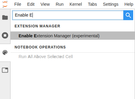
Then, run Jupyter Lab and on the sidebar search for the Extension Manager and enable it, if you haven’t so far.

Image for post
Enable the extension manager

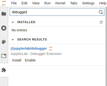
A new button will appear on the sidebar. To install the debugger just go to the newly enabled Extension Manager button and search for the debugger extension.

Image for post
Enable the debugger

After installing it Jupyter Lab will ask you to perform a build to include the latest changes. Accept it, and, after a few seconds, you are good to go.

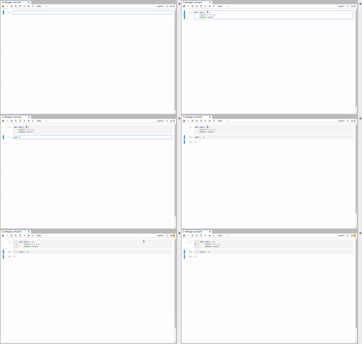
To test the debugger, we create a new xpython notebook and compose a simple function. We run the function as usual and observe the result. To enable the debugger, press the associated button on the top right of the window.

Image for post
Enable the debugger

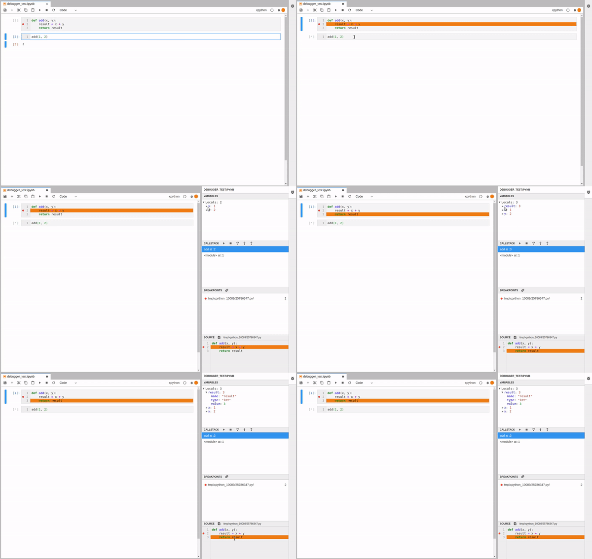
Now, we are ready to run the function again. Only this time the execution will stop at the breakpoint we set and we will be able to explore the state of the program.

Image for post
Debug the code

We see that the program stopped at the breakpoint. Opening the debugger panel we see the variables, a list of breakpoints, the call stack navigation and the source code.

The new visual debugger for Jupyter offers everything you would expect from an IDE debugger. It is still in development, thus, new functionality is expected. Some of the features that its developers plan to release in 2020 are:

  • Support for rich mime type rendering in the variable explorer
  • Support for conditional breakpoints in the UI
  • Enable the debugging of Voilà dashboards, from the JupyterLab Voilà preview extension
  • Enable debugging with as many kernels as possible

Conclusion

Jupyter notebooks have always been a great way to explore and experiment with your code. However, software developers usually turn to a full-fledged IDE, copying the parts that work, to produce a production-ready library.

This is not only inefficient but also a loss on the Jupyter offering; literate programming. Moreover, notebooks provide an environment for better documentation, including graphs, images and videos, and sometimes better tools, such as auto-complete functionality.

nbdev and the visual debugger are two projects that aim at closing the gap between notebooks and IDEs. In this story, we saw what nbdev is and how it makes literate programming a reality. Furthermore, we discovered how a new project, the visual debugger for Jupyter, provides the missing piece.

My name is Dimitris Poulopoulos and I’m a machine learning researcher at BigDataStack and PhD(c) at the University of Piraeus, Greece. I have worked on designing and implementing AI and software solutions for major clients such as the European Commission, Eurostat, IMF, the European Central Bank, OECD, and IKEA. If you are interested in reading more posts about Machine Learning, Deep Learning and Data Science, follow me on Medium, LinkedIn or @james2pl on twitter.

Handling exceptions in Python a cleaner way, using Decorators

Handling exceptions in python can get in some cases repetitive and ugly, we can solve that using decorators.

May 17 · 3 min read
Image for post

Functions in Python

Functions in Python are first class objects, which means they can be assigned to a variable, passed as an argument, and return from another function and store that in any data structure.

def example_function():
print("Example Function called")
some_variable = example_functionsome_variable()
Example Function called

Decorators

The first class object property of function helps us to use the concept of Decorators in Python. Decorators are functions which take as argument another function as an object, which enables us to put our logic either at the start and end of the execution of the argument function.

def decorator_example(func):
print("Decorator called")

def inner_function(*args, **kwargs):
print("Calling the function")
func(*args, **kwargs)
print("Function's execution is over")
return inner_function
@decorator_example
def some_function():
print("Executing the function")
# Function logic goes here
Decorator called
Calling the function
Executing the function
Function's execution is over

Error Handling Using Decorators

You can use Decorators for quite a lot of purposes like logging, validations, or any other common logic which needs to be put in multiple functions. One of the many areas where Decorators can be used is the exception handling.

def area_square(length):
try:
print(length**2)
except TypeError:
print("area_square only takes numbers as the argument")


def area_circle(radius):
try:
print(3.142 * radius**2)
except TypeError:
print("area_circle only takes numbers as the argument")


def area_rectangle(length, breadth):
try:
print(length * breadth)
except TypeError:
print("area_rectangle only takes numbers as the argument")
def exception_handler(func):
def inner_function(*args, **kwargs):
try:
func(*args, **kwargs)
except TypeError:
print(f"{func.__name__} only takes numbers as the argument")
return inner_function


@exception_handler
def area_square(length):
print(length * length)


@exception_handler
def area_circle(radius):
print(3.14 * radius * radius)


@exception_handler
def area_rectangle(length, breadth):
print(length * breadth)


area_square(2)
area_circle(2)
area_rectangle(2, 4)
area_square("some_str")
area_circle("some_other_str")
area_rectangle("some_other_rectangle")
4
12.568
8
area_square only takes numbers as the argument
area_circle only takes numbers as the argument
area_rectangle only takes numbers as the argument

+ Recent posts